Using iterative methods to solve the Laplace equation

Theoretical introduction

The example in this notebook is based on the book [1].

[1] Gabriele Ciaramella and Martin J. Gander. Iterative Methods and Preconditioners for Systems of Linear Equations. 2020.

In this notebook, we will guide you through solving the Laplace equation. Consider the domain \(\Omega = (0,1)^2 \subset \mathbb{R}\) and a function \(g \in C^0(\overline{\Omega})\), we want to find a (strong) solution \(u \in C^2(\overline{\Omega})\) for the following boundary value problem

\[\begin{align*} \Delta u &= 0 \text{ in } \Omega\\ u &= g \text{ on } \partial \Omega. \end{align*}\]

Here \(\Delta = \partial_x^2 + \partial_y^2\) is the Laplace Operator. As we are looking for a strong solution, we start with a finite difference approximation via

\[\begin{align*} \partial_x^2 u(x,y) &\approx \frac{u(x+h, y) - 2u(x,y) + u(x-h,y)}{h^2} \label{eq:DiscretePartialX} \tag{1}\\ \partial_y^2 u(x,y) &\approx \frac{u(x, y+h) - 2u(x,y) + u(x,y-h)}{h^2}\label{eq:DiscretePartialY} \tag{2},\\ \end{align*}\]

for a mesh size \(h = \frac{1}{m+1}> 0\), \(m\in \mathbb{N}\). By defining the grid points \((x_j, y_i) = (jh, ih)\) and summing \eqref{eq:DiscretePartialX} and \eqref{eq:DiscretePartialY}, we obtain

(1)\[\begin{align} u_{i,j-1} + u_{i-1,j} - 4u_{i,j} + u_{i+1,j} + u_{i,j+1} = 0 \label{eq:DiscreteLaplace}\tag{3} \end{align}\]

as an approximation for equation \(\Delta u = 0\). For simplicity, we assume that \(g \equiv 1\) on the set \(\{(x,1) \vert x \in [0,1]\}\) and \(g \equiv 0\) otherwise.

Let us introduce the vectors

\[\begin{align*} \mathbf{u}_j := \begin{pmatrix} u_{1,j}\\ \vdots\\ u_{m,j} \end{pmatrix}, j = 1,2,\ldots, m, \end{align*}\]

which contain the values \(u_{i,j}\) for \(i=1,\ldots, m\) on an vertical column corresponding to \(j\). By rewriting the upper system of linear equations \eqref{eq:DiscreteLaplace} and using the top boundary condition (attention: the boundary conditions are shifted into the right-hand side), where \(u \equiv 1\), we get

\[\begin{align*} \mathbf{u}_{j-1} + T \mathbf{u}_j + \mathbf{u}_{j+1} = - \mathbf{e}_m = -(0,\ldots, 0, 1)^T \in \mathbb{R}^m, \end{align*}\]

with the Matrix

\[\begin{align*} T := \begin{pmatrix} -4 & 1 & & & \\ 1 & -4 & 1 & & \\ & \ddots & \ddots & \ddots & \\ %& & \ddots & \ddots & 1 \\ %& & & 1 & -4 \end{pmatrix} \in\mathbb{R}^{m\times m}. \end{align*}\]

By defining the vector

\[\begin{align*} \mathbf{u} := \begin{pmatrix} \mathbf{u}_1\\ \vdots\\ \mathbf{u}_m \end{pmatrix} \in \mathbb{R}^{m^2}, \end{align*}\]

we obtain the following system of linear equations

\[\begin{align*} A \mathbf{u} = \mathbf{f}. \end{align*}\]

The matrix \(A\) is given by

\[\begin{align*} A = \text{I}_m \otimes T + T \otimes \text{I}_m= \begin{pmatrix} T & \text{I}_m & & \\ \text{I}_m & T & \text{I}_m & \\ & \ddots & \ddots & \ddots \end{pmatrix} \in\mathbb{R}^{m^2\times m^2}, \end{align*}\]

with the Kronecker product \(\otimes\) and the right-hand side \(\mathbf{f}\) containing the boundary conditions. While constructing A, the boundedness of the domain has to be taken into account. In particular, that nodes at the edges do not have 4 neighbouring cells, but three or two.

Let us define the system matrices and the right-hand side. Feel free to change e.g. the mesh size.

import numpy as np
from oppy.tests.itMet import FDLaplacian

# number of grid points
m = 20
# build the system matrix
A = FDLaplacian(m, 2)
# define the right-hand side
f = np.zeros(m**2)
f[m-1:-1:m] = -1
# set the last entry manually
f[-1] = -1

Compute a first solution using the scipy sparse solver

Fist, let us compute the exact solution using the scipy sparse solver.

# enable 3D plotting
import matplotlib.pyplot as plt
from mpl_toolkits.mplot3d import Axes3D
from matplotlib import cm

from scipy.sparse.linalg import spsolve

u_exact = spsolve(A, f)
print('norm of the residual = {}'.format(np.linalg.norm(A.dot(u_exact)-f)))
# we need to reshape the 1D vector back to 2D
U_exact = np.zeros((m+2, m+2))
U_exact[1:m+1, 1:m+1] = np.reshape(u_exact, (m, m))
# manually set the correct boundary conditions
U_exact[0:-1,-1] = 1

x_grid = np.linspace(0,1,m+2)
y_grid = x_grid
# attention, later we need to interchange X,Y
# (see the definition of the vector u)
X, Y = np.meshgrid(x_grid, y_grid)


# plotting
fig = plt.figure(figsize=(10,10))
ax = fig.add_subplot(111, projection='3d')
ax.set_xlabel('x-axis')
ax.set_ylabel('y-axis')
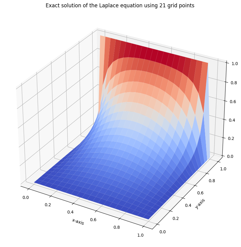
ax.set_title('Exact solution of the Laplace equation using {} grid points'.format(m+1))
surf = ax.plot_surface(Y,X, U_exact, cmap=cm.coolwarm)
plt.show()

norm of the residual = 3.664556843905133e-15

Iterative Solvers

Now we want to use the solvers implemented in oppy to solve the upper system and compare their results. For the reason of comparsion, we run all of the algorithms with their default options and hence, we only define an options object once. We start with the standard iterative solver: Jacobi’s method, Gauss-Seidel method, Successive over-relaxation (SOR) method and the Steepest descent algorithm.

from oppy.itMet import jacobi, gauss_seidel, sor, steepest_descent

from oppy.options import Options

# create a dict to save all results and print them in the end
res_dict = {}

jacobi_options = Options(tol_abs=1e-7, tol_rel=1e-7, nmax=1e5, results='all')
res_dict['jacobi'] = jacobi(A, f, jacobi_options)

gauss_seidel_options = Options(tol_abs=1e-7, tol_rel=1e-7, nmax=1e5, results='all')
res_dict['gauss_seidel'] = gauss_seidel(A, f, gauss_seidel_options)

sor_options = Options(tol_abs=1e-7, tol_rel=1e-7, nmax=1e5, omega=1/2, results='all')
res_dict['sor'] = sor(A, f, sor_options)

steepest_descent_options = Options(tol_abs=1e-7, tol_rel=1e-7, nmax=1e5, results='all')
res_dict['steepest_descent'] = steepest_descent(A, f, steepest_descent_options)

Krylov methods

In order to further improve our results, we want to switch from stationary solvers to more advanced krylov (subspace) methods: the conjugated gradient (CG) method and the generalized minimal residual (GMRES) algorithm. For the reason of comparability, we will keep the same options:

from oppy.itMet import cg, gmres
cg_options = Options(tol_abs=1e-7, tol_rel=1e-7, nmax=1e5, results='all')
res_dict['cg'] = cg(A, f, cg_options)

gmres_options = Options(tol_abs=1e-7, tol_rel=1e-7, nmax=1e5, results='all')
res_dict['gmres'] = gmres(A, f, gmres_options)

Conclusion: Comparison of convergence rates

Let us plot the different convergence behaviours of our methods. In the plot below, you can see the history with the norm of the residuals and plotted against the iteration index.

# Plot the norm of the residual for all methods:
plt.figure(figsize=(15,10))

for key in res_dict:
    plt.semilogy(res_dict[key].res, label = key)
    

plt.legend(loc="upper right")
plt.title('Convergence results for different methods')
plt.xlabel('Number of iterations')
plt.ylabel("Norm of the residual")
plt.show()

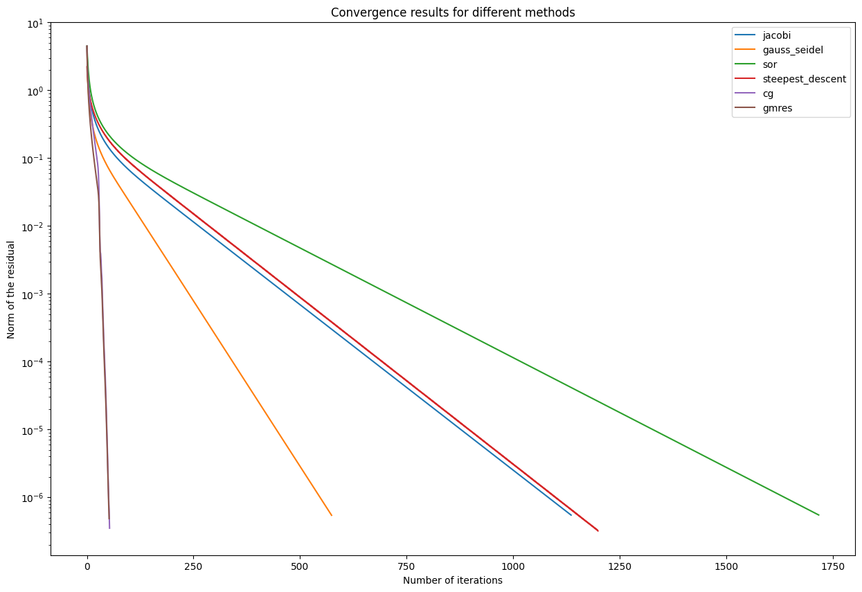
One can see that the Krylov methods provide really good convergence results and a convincing precision.

Krylov methods vs. scipy sparse solver

In order to improve the results even further and compete with the scipy.sparse.linalg.spsolve method, we will increase the precision of our algorithms even more:

# again the scipy solution
u_exact = spsolve(A, f)
print('norm of the residual (scipy) = {}'.format(np.linalg.norm(A.dot(u_exact)-f)))

# cg with maximum precision
cg_options_prec = Options(tol_abs=1e-20, tol_rel=1e-20, nmax=1e5, results='all')
res_cg_prec = cg(A, f, cg_options_prec)
print('norm of the residual (cg) = {}'.format(
    np.linalg.norm(A@res_cg_prec.x - f)))

# gmres with maximum precision
gmres_options_prec = Options(tol_abs=1e-20, tol_rel=1e-20, nmax=1e5, results='all')
res_gmres_prec = gmres(A, f, gmres_options_prec)
print('norm of the residual (gmres) = {}'.format(
    np.linalg.norm(A@res_gmres_prec.x - f)))

norm of the residual (scipy) = 3.664556843905133e-15
norm of the residual (cg) = 1.1240026711206586e-14

norm of the residual (gmres) = 5.918863947170017e-14

This result is really good. Our algorithms are able to yield results in the order of the scipy.sparse.linalg.spsolve algorithm and thus convincing precision. Feel free to play around with the relative and absolute tolerances, as well as the maximum number of iterations.