Solve a Lotka-Volterra based ODE Optimal Control Problem

Notebook to demonstrate how to solve a Lotka-Volterra optimal control via oppy

We consider the Lotka-Volterra optimal control problem

\[\begin{align*} &\min_{y,u}J(y,u)\\ &\mathrm{s.t.}\begin{cases}\, &\dot{y}_1(t)&=ay_1(t)-dy_1(t)y_2(t) +u(t)&\quad \mathrm{in}\,t\in(0,T)\quad\mathrm{with}\quad y_1(0)=y^0_1>0,\\ &\dot{y}_2(t)&=-by_2(t)+cy_1(t)y_2(t)&\quad \mathrm{in}\,t\in(0,T)\quad \mathrm{with}\quad y_2(0)=y^0_2>0,\end{cases} \end{align*}\]

where \(J(y,u)=-(y_1(T)+y_2(T))+\frac{\nu}{2}\int_0^T|u(t)|^2dt,\) is the costfunctional, \(u\in U_{ad}:=\{x\in L^2(0,T;\mathbb{R}) \,: \,0\leq x(t)\leq 1\}\) is the control function, \(y= [y_1,y_2]^T\) is the solution of the state equation, \(a,b,c\) are model parameters and \(\nu\) a regularization parameter.

For implementation purpose we use the following equivalent formulation of the state equation:

\[\begin{align*} \dot{y}=Ay+F(y)+uB, \end{align*}\]

where \(A=\left(\begin{array}{ c c} a&0\\ 0&-b\end{array}\right)\), \(F=\left(\begin{array}{c} -dy_1y_2\\ cy_1y_2\end{array}\right)\) and \(B=\left(\begin{array}{ c } 1\\ 0\end{array}\right)\)

To approach this problem we define the reduced cost functional:

\[\begin{align*} \hat{J}(u)=J(\mathcal{S}(u),u), \end{align*}\]

where \(\mathcal{S}\) is the solution operator which means \(y=\mathcal{S}(u)\) solves the differntial equation in the constraints with the corresponding control \(u\). One can show that solving the reduced problem is equivalent to the original problem (see [1], Chapter 3.1).

The idea is to use an constrained optimization method on the reduced problem. Therefore, following the Lagrange method (see [1], Chapter 4.1) we derive the gradient condition for computing the optimal solution \((\hat{y},\hat{u})\) of the linear quadratic optimal control problem:

\[\begin{align*} \nabla \hat{J}(\hat{u})= \nu \hat{u}+B^T\hat{p}=0, \end{align*}\]

where \(\hat{p}\) solves the adjoint equation:

\[\begin{align*} \begin{array}{r l r} -\dot{p}(t)&=A^Tp(t)+J_F(\hat{y}(t))^Tp(t),&\mathrm{for}\,t\in[0,T],\\ p(T)&=-(y_1(T)+y_2(T))&\end{array}, \end{align*}\]

where \(J_F(\hat{y}(t))\) is the Jacobian matrix of \(F\) evaluated at \(\hat{y}(t)\).

Moreover for evaluating the reduced cost functional \(\hat{J}(u)\) we solve the differential equation in the constraints by integrating forward and for computing the reduced gradient (if required) \(\nabla\hat{J}(u)\) we integrate the adjoint equation backwards. These algorithms are written in a seperate file called \(\small{\textbf{functions.py}}\).

The parameter data for the Lotka-Volterra problem as well as the option parameters for the linesearch and the options of the optimization methods are written in the \(\small{\textbf{problem_data.py}}\) and thus have to be imported.

[1] Gabriele Ciaramella, Script lecture: \(\scriptsize{\textit{Optimal Control of Ordinary Differential Equations}}\), July 21, 2019.

First let’s import all dependencies needed.

import numpy as np

from oppy.options import Options
from oppy.conOpt import projected_gradient

import functions_lotka_volterra as fun
import problem_data_lotka_volterra as data

import matplotlib.pyplot as plt

Now we define the initial control function, the lower and upper boundaries, the reduced cost functional and its derivatives for the optimization method. Furthermore the Armijo Goldstein and Projected Armijo linesearch are defined with optional options.

# Lower boundaries:
a = np.array([0])

# Upper boundaries:
b = np.array([1])

# Define cost function and derivatives
def fhandle(x):
    f = fun.FG(x,data.time,data,1)
    return f

def dfhandle(x):
    f, grad, y, p = fun.FG(x,data.time,data.data,4)
    return grad

Now we set the optional options for the optimization methods. Here we define the options for the Gradient, L-BFGS and the Newton method, where we also use different norm formulas. For comparison purposes we define for each optimization methods a Armijo Goldstein and a projected Armijo linesearch.

# Define norm for projected Gradient
def norm(x,d):
    nor = np.linalg.norm(x-np.clip(x-d, a, b))**2*data.diff[0]
    return nor

def normNewton(x,x_1):
    return data.diff[0]*np.abs(np.sum((x-x_1)))**2

Finally we can run the optimization methods with an random initial control \(u\in\mathbb{R}^{N}\)

# Random initial guess
u0 = np.random.rand(data.N)

# Options for Projected Gradient
options_proj_grad_armijo_gold = Options(norm = norm, disp=True)

# Projected gradient scheme
result_proj_grad = projected_gradient(fhandle, dfhandle, u0, a, b, options_proj_grad_armijo_gold)
residual_proj_grad = result_proj_grad.res

| Iteration | Function value | Step size  |     Residual     |
| it =    1 | f =    -2.3142 | t = 1.0000 | res = 4.7382e-02 |
| it =    2 | f =    -2.3319 | t = 0.5000 | res = 9.7854e-04 |
| it =    3 | f =    -2.3326 | t = 1.0000 | res = 4.4742e-06 |
| it =    4 | f =    -2.3326 | t = 1.0000 | res = 1.2017e-06 |
| it =    5 | f =    -2.3326 | t = 0.5000 | res = 2.5567e-08 |

The projected gradient terminates at 5 iterations. To reach a faster convergence we consider the L-BFGS-B method.

from oppy.conOpt import l_bfgs_b

# Set options for L-BFGS-B scheme
options_l_bfgs_b = Options(norm = norm, disp=True)

# L-BFGS-B scheme
result_l_bfgs_b = l_bfgs_b(fhandle, dfhandle, u0, a, b, options_l_bfgs_b)
residual_l_bfgs_b = result_l_bfgs_b.res

| Iteration | Function value | Step size  |     Residual     |
| it =    1 | f =    -1.0436 | t = 1.0000 | res = 4.7382e-02 |
| it =    2 | f =    -2.3142 | t = 0.5000 | res = 3.3940e-03 |
| it =    3 | f =    -2.3308 | t = 1.0000 | res = 9.5772e-05 |
| it =    4 | f =    -2.3325 | t = 1.0000 | res = 1.3002e-06 |
| it =    5 | f =    -2.3326 | t = 1.0000 | res = 1.3853e-08 |

The L-BFGS-B method terminates at 6 iterations, which means that this method with default options is slightly slower than the projected gradient method. We try another method which is called the projected Newton method. Therefore we define the action of the hessian of the costfunction. Thereafter we define the options of the projected Newton method and execute the algorithm.

from oppy.conOpt import projected_newton

def ddfhandle(x, u, Active, Inactive):
    J, grad, y, p = fun.FG(u,data.time,data.data,4)
    RAct = fun.Hessian(x, u, y, p, data.time, Active, Inactive, data.data, 1)
    return RAct

# Set options for Projected Newton scheme
options_proj_newton = Options(norm = normNewton, disp=True)

# Projected Newton scheme
result_proj_newton = projected_newton(fhandle, dfhandle, ddfhandle, u0, a, b, options_proj_newton)
residual_proj_newton = result_proj_newton.res

| Iteration | Function value | Step size  |     Residual     |
| it =    1 | f =    -2.3304 | t = 1.0000 | res = 7.0255e-02 |

| it =    2 | f =    -2.3326 | t = 1.0000 | res = 1.1522e-02 |

| it =    3 | f =    -2.3326 | t = 1.0000 | res = 9.5370e-04 |

| it =    4 | f =    -2.3326 | t = 1.0000 | res = 7.4697e-09 |

This method needs 5 iterations steps to terminate like the projected gradient method. An error plot with respect to iteration numbers of the different optimization methods with a semi y-axis log scale is used to compare the different schemes.

# Plot convergence rate
plt.semilogy(residual_proj_grad, label='Projected Gradient')
plt.semilogy(residual_l_bfgs_b, label='L_BFGS_B')
plt.semilogy(residual_proj_newton, label='Projected Newton' )
plt.title('Norm of the gradient, different schemes')
plt.grid(True)
plt.legend()
plt.show()

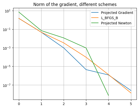
All methods converge within 6 iterations. In this Lotka Volterra optimal problem the projected Newton method with default options provides the best solution, since it terminates at 5 iterations with the lowest residual value.

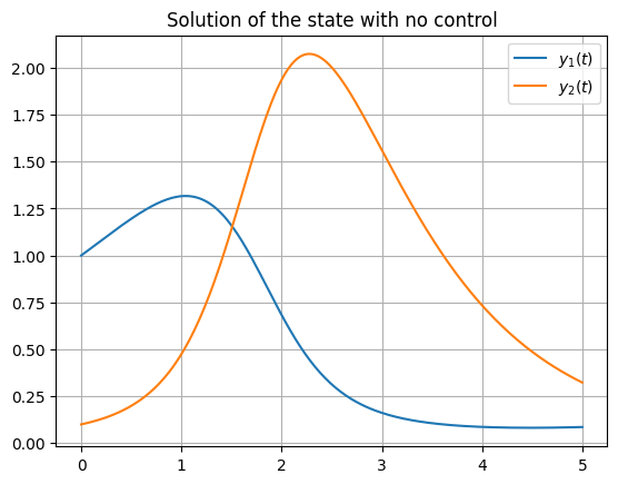
For better understanding of the problem, we plot the states \(y\) without a control function \(u\) with respect to the time \(t\).

# Plot uncontrolled state
u0 = np.zeros((data.N,))
f_0 , grad_0 , y_0 , p_0 = fun.FG( u0 , data.time, data.data , 4 )

xAxe = np.linspace(0,data.T, num=data.N)
plt.plot(xAxe,y_0[0,:], label='$y_1(t)$')
plt.plot(xAxe,y_0[1,:], label='$y_2(t)$')
plt.title('Solution of the state with no control')
plt.grid(True)
plt.legend()
plt.show()

We will now extract the optimal solution of the results of the quasi Newton method and solve the differential equation, which is the constraint of the optimal control problem. Therefore we use the forward solver.

# Plot optimal solution
f1 , grad , y , p = fun.FG( result_proj_newton.x , data.time, data.data , 4 )
xAxe = np.linspace(0,data.T, num=data.N)
plt.plot(xAxe,y[0,:], label='$y_1$')
plt.plot(xAxe,y[1,:], label='$y_2$')
plt.plot(xAxe, result_proj_newton.x, label='$u(t)$')
plt.xlabel('time')
plt.ylabel('prey $y_1(t)$ and predators $y_2(t)$')
plt.title('Optimal Solution')
plt.grid(True)
plt.legend()
plt.show()

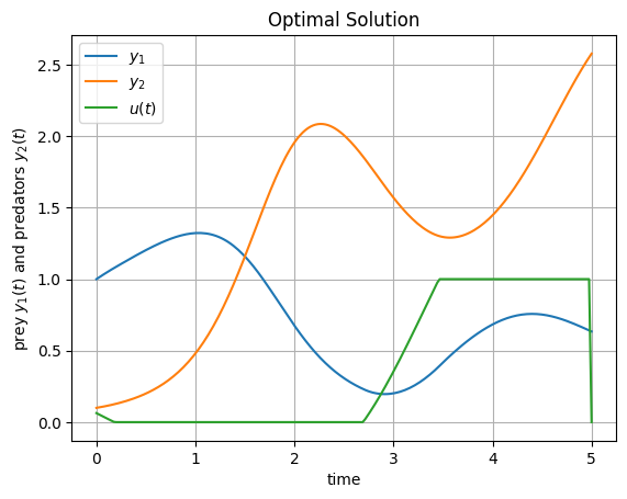
The state outcome with optimal control aligns with the optimal control problem since the costfunction aims to maximize the states in each variable.