Solving a Convex Multiobjective Optimization Problem

Given the vector-valued objective function \(f:\mathbb{R}^2\to \mathbb{R}^3\), we consider the following multiobjective optimization problem (MOP)

\[\begin{equation*} \begin{gathered}%\label{eq:P}\tag{P} \min\limits_{x\in \mathbb{R}^2} f(x) = \left( \begin{array} \vert \| x-v_1\|^2_2\\ \|x-v_2\|^2_2\\ \|x-v_3\|^2_2 \end{array} \right)\\ \begin{alignedat}{3} \mbox{s.t. } -2 \leq x_i \leq 2 \quad \forall i\in\{1,2\}. \end{alignedat} \end{gathered} \end{equation*}\]

Further, we set the vertices of the three parabolas as \(v_1=[1,1]^T,\ v_2=[-0.5,-1]^T\) and \(v_3=[1.5,-1.5]^T\) and \(\|\cdot\|_2\) denotes the euclidian distance in \(\mathbb{R}^2\).

Since all components of the objective function \(f\) and the costraints are convex, the MOP is convex, which implies that the Pareto set consists of one connected component. Further, it will turn out that the Pareto set consists of the convex hull of the points \(v_1,\ v_2,\ v_3\). For convex MOPs the weighted-sum method (WSM) and euclidian reference point are well suited and their application on the MOP will be demonstrated below.

At first, we load the modules, define the objective function and its derivatives and store them in a list.

import numpy as np
from oppy.multOpt.mop import solve_MultiobjectiveOptimizationProblem
import matplotlib.pyplot as plt
from oppy.options import Options
from oppy.conOpt import projected_armijo, projected_gradient

# Specify the vertices of the parabolas
v1 = np.array([1, 1])
v2 = np.array([-0.5, -1])
v3 = np.array([1.5, -1.5])

# Define the cost functions
f1 = (lambda x: (x[0] - v1[0])**2 + (x[1] - v1[1])**2)
f2 = (lambda x: (x[0] - v2[0])**2 + (x[1] - v2[1])**2)
f3 = (lambda x: (x[0] - v3[0])**2 + (x[1] - v3[1])**2)

# Define the gradients
df1 = (lambda x: np.array([2*(x[0] - v1[0]), 2*(x[1] - v1[1])]))
df2 = (lambda x: np.array([2*(x[0] - v2[0]), 2*(x[1] - v2[1])]))
df3 = (lambda x: np.array([2*(x[0] - v3[0]), 2*(x[1] - v3[1])]))

# Define the Hessians
ddf1 = (lambda x: np.array([[2, 0], [0, 2]]))
ddf2 = (lambda x: np.array([[2, 0], [0, 2]]))
ddf3 = (lambda x: np.array([[2, 0], [0, 2]]))

# Store the cost functions, their gradients and Hessians in a list
f = [f1, f2, f3] 
df = [df1, df2, df3] 
ddf = [ddf1, ddf2, ddf3]

Next, we define the lower and upper bounds for the box constraints and the initial value for the minimization of the first scalar subproblem.

# Define the box constraints
low = np.array([-2, -2])
up = np.array([2, 2])

# Set the initial value
x = np.array([0, 0])

Solution with the Weighted-Sum Method (WSM)

First, we want to solve the convex MOP with the WSM. In order to do that we define the following options for the optimization. We choose the projected Gradient method with an Armijo line search as an inner solver for the scalar subproblems. Note that the only possibility to define a line search for the inner solver is the way, which is depicted below. Further, we set number of weights per dimension to 30 and mark the problem type as convex to improve the efficiency of the solver.

# Define the solver function for the scalar subproblems
def optimeth_proj_grad(fhandle, dfhandle, x, low, up, ddfhandle=None):
    
    # Define line search
    def linesearch_inner_proj_armijo(x, d, low, up):  
        t, flag = projected_armijo(fhandle, x, d, low, up, options=None)
        return t, flag
    
    # Set the options
    options_proj_grad = Options(nmax=1000,
                                disp=False, stop=False, statusdisp=True,
                                linesearch=linesearch_inner_proj_armijo)
    
    # Apply the optimization algorithm
    result_opt = projected_gradient(fhandle, dfhandle, x, low, up,
                                    options_proj_grad)
    return result_opt

# Define the options for the WSM
options_mop_WSM = Options(mop_method="WSM", num_weights_per_dimension=30,
                          WSM_optimeth=optimeth_proj_grad,
                          problem_type="convex")

Now we are ready to solve the MOP with the WSM and save the Pareto set and the functional values of the objectives.

# Solve the Multiobjective Optimization Problem with the WSM
MOP, data = solve_MultiobjectiveOptimizationProblem(f, df, x, low, up,
                                                    options_mop_WSM)

# Get the Pareto set
x_opt = MOP["1,2,3"].x 

# Get the Pareto front
f_values = MOP["1,2,3"].func_values

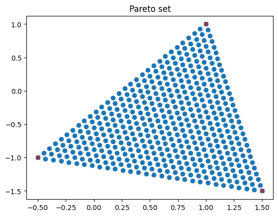
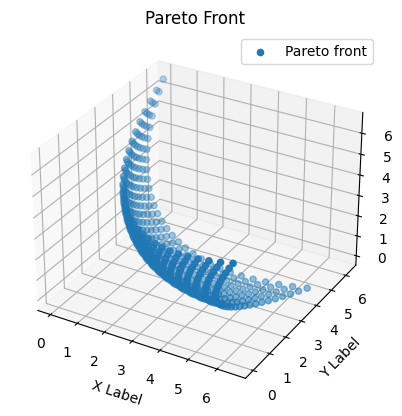
Now we can plot the resulting Pareto set and the Pareto front. Note that the Pareto set is given as the convex hull of \(v_1,v_2,v_3\).

# Plot the Pareto optimal parameters and the points v_i
fig = plt.figure()
plt.title("Pareto set")
plt.plot(x_opt[:, 0], x_opt[:, 1], 'o')
plt.plot(v1[0], v1[1], 'rx')
plt.plot(v2[0], v2[1], 'rx')
plt.plot(v3[0], v3[1], 'rx')
plt.show()

# Plot the Pareto front
fig = plt.figure()
ax = fig.add_subplot(projection='3d')
plt.title("Pareto Front")
ax.scatter(f_values[:, 0], f_values[:, 1], f_values[:, 2], 'o',label='Pareto front')
ax.legend(loc='best')
ax.set_xlabel('X Label')
ax.set_ylabel('Y Label')
ax.set_zlabel('Z Label')

plt.show()

Solution with Euclidian Reference Point Method (ERPM)

Next, we solve the problem using the ERPM. We specify the following options, where we set \(h_p=0.2\) and \(h_x=0.8\). Again we choose the Projected Gradient method as an inner solver for the scalar subproblems and set the problem type to convex.

# Define the options for the ERPM
options_mop_ERPM = Options(mop_method="ERPM", hp=0.2, hx=0.8,                          
                           ERPM_optimeth=optimeth_proj_grad,
                           problem_type="convex")

Now we are ready to solve again and save the computed Pareto set, the Pareto front and all computed reference points:

# Solve the Multiobjective Optimization Problem with the ERPM
MOP, data = solve_MultiobjectiveOptimizationProblem(f, df, x, low, up,
                                                    options_mop_ERPM)

# Get the Pareto set
x_opt = MOP["1,2,3"].x

# Get the Pareto front
f_values = MOP["1,2,3"].func_values

# Get the reference points
z_ref = MOP["1,2,3"].z_ref_all

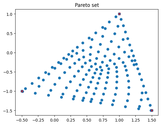
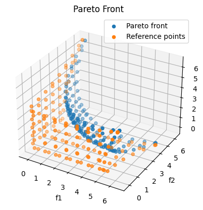
Finally we plot the obtained results:

# Plot the Pareto optimal parameters
fig = plt.figure()
plt.title("Pareto set")
plt.plot(x_opt[:, 0], x_opt[:, 1], 'o')
plt.plot(v1[0], v1[1], 'rx')
plt.plot(v2[0], v2[1], 'rx')
plt.plot(v3[0], v3[1], 'rx')
plt.show()

fig = plt.figure()
ax = fig.add_subplot(projection='3d')
plt.title("Pareto Front")
ax.scatter(f_values[:, 0], f_values[:, 1], f_values[:, 2], 'o',label='Pareto front')
ax.scatter(z_ref[:, 0], z_ref[:, 1], z_ref[:, 2], 'o', label='Reference points')
ax.legend(loc='best')
ax.set_xlabel('f1')
ax.set_ylabel('f2')
ax.set_zlabel('f3')
plt.show()