Multiojective Optimization of the Fonseca Fleming function

For \(n\in \mathbb{N}\), we consider the box-constrained bicriterial optimization of the Fonseca-Fleming function

\[\begin{equation*} \begin{gathered}%\label{eq:P}\tag{P} \min\limits_{x\in \mathbb{R}^n} f(x)=\left( \begin{array}{c} 1-\exp\bigg(-\sum\limits_{i=1}^n\Big(x_i-\frac{1}{\sqrt{n}}\Big) ^2\bigg)\\ 1-\exp\bigg(-\sum\limits_{i=1}^n\Big(x_i+\frac{1}{\sqrt{n}}\Big)^2\bigg) \end{array} \right)\\ \begin{alignedat}{3} \mbox{s.t. } -2 \leq x_i \leq 2 \quad \forall i\in\{1,\ldots,n\}. \end{alignedat} \end{gathered} \end{equation*}\]

This is a non-convex MOP since the objective function is not convex. For these types of problems the canonical choice of our optimization package is the Pascoletti-Serafini method (PSM), which will give the best results. We will see that the WSM cannot compute the Pareto set in this case. However the ERPM can compute the Pareto front, but not in an uniformly discretized manner.

First, we import the modules:

import numpy as np
from oppy.multOpt.mop import solve_MultiobjectiveOptimizationProblem
import matplotlib.pyplot as plt
from oppy.options import Options
from oppy.conOpt import l_bfgs_b, augmented_lagrangian, projected_armijo, projected_gradient

Next, we set \(n=2\) for simplicity, specify the cost functions and their derivatives and store them in a list:

# Set n
n = 2

# Define the cost functions
def f1(x):
    exponent = 0
    for i in range(n):
        exponent -= (x[i] - 1/np.sqrt(n))**2
    return 1 - np.exp(exponent)


def f2(x):
    exponent = 0
    for i in range(n):
        exponent -= (x[i] + 1/np.sqrt(n))**2
    return 1 - np.exp(exponent)

# Define the derivatives
def df1(x):
    grad_val = np.zeros(x.shape[0])
    exponent = 0
    for i in range(x.shape[0]):
        exponent -= (x[i] - 1/np.sqrt(n))**2
    for i in range(x.shape[0]):
        grad_val[i] = 2*(x[i] - 1/np.sqrt(n)) * np.exp(exponent)
    return grad_val


def df2(x):
    grad_val = np.zeros(x.shape[0])
    exponent = 0
    for i in range(x.shape[0]):
        exponent -= (x[i] + 1/np.sqrt(n))**2
    for i in range(x.shape[0]):
        grad_val[i] = 2*(x[i] + 1/np.sqrt(n)) * np.exp(exponent)
    return grad_val


# Define the Hessians
ddf1 = (lambda x: np.array([[2, 0], [0, 2]]))
ddf2 = (lambda x: np.array([[2, 0], [0, 2]]))

# Store the cost functions, their gradients and Hessians in a list
f = [f1, f2]  
df = [df1, df2] 
ddf = [ddf1, ddf2] 

Further, we set the box constraints and define the initial guess for the solution of the first subproblem.

# Define the box constraints
low = np.array([-2, -2])
up = np.array([2, 2])

# Set the initial value for the solution of the first subproblem
x = np.array([0, 0])

Solution with the Pascoletti-Serafini method (PSM)

We want to solve the problem with the PSM. As an solver for the scalar subproblems of the PSM we choose the Augmented Lagrange method. Note that we need to extend the bounds for the Augmented Lagrangian, since it also approximates the multiplier of the box constraints and further the Augmented Lagrange method uses an inner solver, for which we choose the L-BFGS algorithm. The whole procedure is depicted below:

# Extend the box constraints for the augmented Lagrange
low_aug = np.hstack((low, -np.Inf)) 
up_aug = np.hstack((up, np.Inf))

# Inner optimization for the augmented Lagrangian algorithm
def optimeth_inner_opt_aug_lagr(x, fhandle, dfhandle, eps):
    # Define the line search algorithm
    def default_linesearch(x, d, low, up):
        t, flag = projected_armijo(fhandle, x, d, low, up, options=None)
        return t, flag
    # Set the options
    options_l_bfgs = Options(tol_abs=eps, tol_rel=eps,
                             linesearch=default_linesearch)
    # Apply the optimization algorithm
    result_opt = l_bfgs_b(fhandle, dfhandle, x, low_aug, up_aug,
                          options=options_l_bfgs)
    return result_opt


# Outer optimization algorithm for the Pascoletti-Serafini problems (Augmented
# Lagrangian algorithm)
def optimeth_augm_lagr(fhandle, dfhandle, ghandle, dghandle, x,
                       ddfhandle=None, ddghandle=None):
    # Set the options
    options_augm_lagr = Options(optimeth=optimeth_inner_opt_aug_lagr)
    # Apply the optimization algorithm
    result_opt = augmented_lagrangian(fhandle, dfhandle,
                                      ghandle=ghandle,
                                      dghandle=dghandle, x=x,
                                      options=options_augm_lagr)
    return result_opt

All in all, we specify the following options and set the problem_type to non-convex.

# Set the options for the PSM
options_mop_PSM = Options(mop_method="PSM", hp=0.2, hx=0.05,
                          r_PSM=np.ones(len(f)),                         
                          PSM_optimeth=optimeth_augm_lagr,
                          problem_type="non-convex")

Now we are ready to solve and store the computed data:

# Solve the Multiobjective Optimization Problem with the PSM
MOP, data = solve_MultiobjectiveOptimizationProblem(f, df, x, low, up,
                                                    options_mop_PSM)
# Get the Pareto optimal parameters
x_opt = MOP["1,2"].x

# Get the Pareto front
f_values = MOP["1,2"].func_values

# Get the reference points
z_ref = MOP["1,2"].z_ref_all

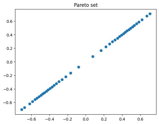
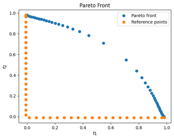
Next, we plot the computed Pareto set and the Pareto front with all reference points.

# Plot the Pareto set
fig = plt.figure()
plt.title("Pareto set")
plt.plot(x_opt[:, 0], x_opt[:, 1], 'o')
plt.show()

# Plot the Pareto front and the reference points
fig = plt.figure()
plt.title("Pareto Front")
plt.plot(f_values[:, 0], f_values[:, 1], 'o',label='Pareto front')
plt.plot(z_ref[:, 0], z_ref[:, 1], 'o',label='Reference points')
plt.legend(loc='best')
plt.xlabel('f1')
plt.ylabel('f2')
plt.show()

We observe that the PSM computes the Pareto set and the discretization of the Pareto front is uniformly.

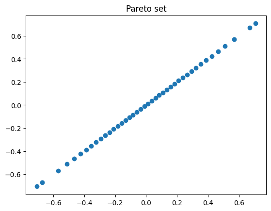
Solution with Euclidian Reference Point Method (ERPM)

Next, we try to solve the problem using the ERPM. Note that from a theoretical point of view, the ERPM fits only for convex problems. However, in this special case we can compute the Pareto front, but not homogeneously discretized.

We define the Projected Gradient method as an inner solver for the ERPM and choose the following options:

# Define the Projected Gradient method as an inner solver for the ERPM
def optimeth_proj_grad(fhandle, dfhandle, x, low, up, ddfhandle=None):
    def linesearch_inner_proj_armijo(x, d, low, up):
        t, flag = projected_armijo(fhandle, x, d, low, up, options=None)
        return t, flag
    options_proj_grad = Options(nmax=1000,
                                disp=False, stop=False, statusdisp=True,
                                linesearch=linesearch_inner_proj_armijo)
    result_opt = projected_gradient(fhandle, dfhandle, x, low, up,
                                    options_proj_grad)
    return result_opt

# Options for the ERPM
options_mop_ERPM = Options(mop_method="ERPM", hp=0.01, hx=0.05,
                           ERPM_optimeth=optimeth_proj_grad,
                           problem_type="non-convex")

We are ready to solve the problem and store the computed data:

# Solve the problem with the ERPM
MOP, data = solve_MultiobjectiveOptimizationProblem(f, df, x, low, up,
                                                    options_mop_ERPM)

# Get the Pareto optimal parameters
x_opt = MOP["1,2"].x

# Get the Pareto front
f_values = MOP["1,2"].func_values

# Get the reference points
z_ref = MOP["1,2"].z_ref_all

And we plot the results:

# Plot the Pareto set
fig = plt.figure()
plt.title("Pareto set")
plt.plot(x_opt[:, 0], x_opt[:, 1], 'o')
plt.show()

# Plot the Pareto front and the reference points
fig = plt.figure()
plt.title("Pareto Front")
plt.plot(f_values[:, 0], f_values[:, 1], 'o',label='Pareto front')
plt.plot(z_ref[:, 0], z_ref[:, 1], 'o',label='Reference points')
plt.legend(loc='best')
plt.xlabel('f1')
plt.ylabel('f2')
plt.show()

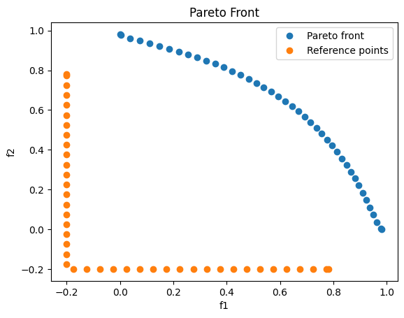
One can see the structure of the Pareto front, but the ERPM fails in discretizing the Pareto front homogeneously.

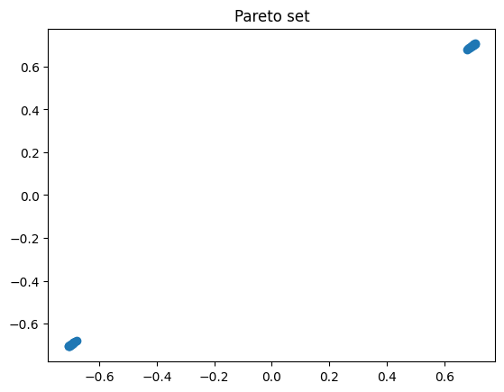
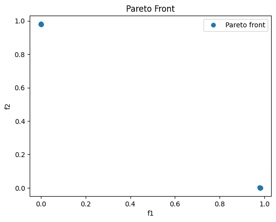
Solution with Weighted-Sum Method (WSM)

This example should indicate what can go wrong when using the WSM to solve a non-convex problem. We specify the following options and solve the problem:

# Specify options for the WSM
options_mop_WSM = Options(mop_method="WSM", num_weights_per_dimension=30,
                          WSM_optimeth=optimeth_proj_grad,
                          problem_type="non-convex")

# Solve the MOP with the WSM
MOP, data = solve_MultiobjectiveOptimizationProblem(f, df, x, low, up,
                                                    options_mop_WSM)

# Get the Pareto optimal parameters
x_opt = MOP["1,2"].x

# Get the Pareto front
f_values = MOP["1,2"].func_values

Finally we plot the results. We observe that the WSM fails to compute the Pareto set/front. Therefore one should pay attention when using the WSM for solving non-convex problems.

# Plot the Pareto optimal parameters
fig = plt.figure()
plt.title("Pareto set")
plt.plot(x_opt[:, 0], x_opt[:, 1], 'o')
plt.show()

# Plot the Pareto front and the reference points
fig = plt.figure()
plt.title("Pareto Front")
plt.plot(f_values[:, 0], f_values[:, 1], 'o',label='Pareto front')
plt.legend(loc='best')
plt.xlabel('f1')
plt.ylabel('f2')
plt.show()