Solve a linear-quadratic ODE Optimal Control Problem
Notebook to demonstrate how to solve an linear quadratic optimal control problem via oppy
We consider the linear quadratic optimal control problem
where \(J(y,u)=\frac{1}{2}||y(T)-y_T||^2+\frac{\mu}{2}||y(t)-y_d(t)||^2+\frac{\nu}{2}||u(t)||^2\) is the costfunctional, \(u\in L^2(0,T;\mathbb{R^m})\) is the control function, \(y\) is the solution of the state equation, \(y_T=[0,1]^T\) is the desired final state, \(y_d\equiv[1,1]^T\) desired trajectory and \(\mu,\nu\) regularization parameters.
To approach this problem we define the reduced cost functional:
where \(\mathcal{S}\) is the solution operator, which means \(y=\mathcal{S}(u)\) solves the differntial equation in the constraints with the corresponding control \(u\). One can show that solving the reduced problem is equivalent to the original problem (see [1], Chapter 3.1).
The idea is to use an unconstrained optimization method on the reduced problem. Therefore, following the Lagrange method (see [1], Chapter 4.1) we derive the gradient condition for computing the optimal solution \((\hat{y},\hat{u})\) of the linear quadratic optimal control problem:
where \(\hat{p}\) solves the adjoint equation:
Moreover for evaluating the reduced cost functional \(\hat{J}(u)\) we solve the differential equation in the constraints by integrating forward and for computing the reduced gradient (if required) \(\nabla\hat{J}(u)\) we integrate the adjoint equation backwards. These algorithms are written in a seperate file called \(\small{\textbf{functions.py}}\).
The parameter data for the linear quadratic problem are written in the \(\small{\textbf{problem_data.py}}\) and thus have to be imported.
[1] Gabriele Ciaramella, Lecture Notes: \(\scriptsize{\textit{Optimal Control of Ordinary Differential Equations}}\), July 21, 2019.
First let’s import all dependencies needed.
import numpy as np

from oppy.options import Options
from oppy.unconOpt import gradmethod
from oppy.unconOpt import armijo

import functions_linear_quadratic as fun
import problem_data_linear_quadratic as data

import matplotlib.pyplot as plt
Now we define the linesearch methods Armijo and Wolfe for the Gradient method, Quasi Newton method and Fletcher Reeves method. Therefore the reduced cost functional and its first derivation is required which is given by \(\texttt{fun.fAndG}\).
Note: The parameters \(y_0, y_T\) are in \(\mathbb{R}^M\) and the matrix \(y_d\in\mathbb{R}^{M\times N}\) are the values of a time dependent function on an equidistant grid with mesh size \(dt\), where \(M\) is the dimension number in space and \(N\) is the number of discretization points.
Moreover, take care that oppy requires one dimensional arrays as input functions!
# Define cost function
def fhandle(x):
    # Check the shape of x
    if x.ndim == 1:
        x = np.reshape(x,(data.M, data.N))
    f = fun.fAndG(x, data.data, 1)
    return f

def dfhandle(x):
    if x.ndim == 1:
        x = np.reshape(x,(data.M, data.N))
    f,grad = fun.fAndG(x, data.data,2)
    grad = np.reshape(grad, (data.M* data.N))
    return grad

# Armijo and Wolfe linesearch options
initstep = 1
beta = 0.5
amax = 30
c1 = 1e-4
c2 = 0.4

options_arm = Options(initstep=initstep, c1=c1, beta=beta, nmax=amax)
options_wol = Options(initstep=initstep, c1=c1, c2=c2, beta=beta, nmax=amax)

def lineNorm(x,d):
    nor = data.dt*np.sum(np.sum(dfhandle(x)*d))
    return nor

# Define Armijo linesearch
def linesearch_armijo(x, d):
    t, flag = armijo(fhandle, dfhandle, x, d, options_arm)
    return t, flag
Now we have to set the options for the optimization methods. The standard discretized \(L_2\)-norm has been chosen for this problem and for all optimization methods. Furthermore the options with armijo or wolfe line search has to be set separately and the Symmetric Rank 1 update method for the Quasi Newton method is used.
# Options for Gradient scheme with Armijo linesearch
opt_grad_armijo = Options(disp=True, linesearch=linesearch_armijo)

# Initial guess
u0 = np.random.rand(data.M*data.N)
Finally we can run the optimization methods with an random initial control \(u\in\mathbb{R}^{M\times N}\). For plotting purpose we reshape the final solution.
# Gradient scheme with Armijo
result_grad_arm = gradmethod(fhandle, dfhandle, u0, opt_grad_armijo)
res_grad_arm = result_grad_arm.res
| Iteration | Function value | Step size  |     Residual     |
| it =    1 | f =     5.4133 | t = 1.0000 | res = 6.7902e+01 |
| it =    2 | f =     4.6948 | t = 1.0000 | res = 6.1462e+01 |
| it =    3 | f =     4.0415 | t = 1.0000 | res = 5.5037e+01 |
| it =    4 | f =     3.4531 | t = 1.0000 | res = 4.8631e+01 |
| it =    5 | f =     2.9296 | t = 1.0000 | res = 4.2251e+01 |
| it =    6 | f =     2.4706 | t = 1.0000 | res = 3.5909e+01 |
| it =    7 | f =     2.0759 | t = 1.0000 | res = 2.9624e+01 |
| it =    8 | f =     1.7451 | t = 1.0000 | res = 2.3434e+01 |
| it =    9 | f =     1.4772 | t = 1.0000 | res = 1.7414e+01 |
| Iteration | Function value | Step size  |     Residual     |
| it =   10 | f =     1.2713 | t = 1.0000 | res = 1.1753e+01 |
| it =   11 | f =     1.1247 | t = 1.0000 | res = 7.0077e+00 |
| it =   12 | f =     1.0320 | t = 1.0000 | res = 4.4986e+00 |
| it =   13 | f =     0.9782 | t = 1.0000 | res = 3.3622e+00 |
| it =   14 | f =     0.9386 | t = 1.0000 | res = 2.2385e+00 |
| it =   15 | f =     0.9104 | t = 1.0000 | res = 1.1489e+00 |
| it =   16 | f =     0.8936 | t = 1.0000 | res = 1.1947e+00 |
| it =   17 | f =     0.8889 | t = 0.2500 | res = 4.4041e-01 |
| it =   18 | f =     0.8879 | t = 0.1250 | res = 3.7231e-01 |
| it =   19 | f =     0.8879 | t = 0.0625 | res = 5.8974e-02 |
| Iteration | Function value | Step size  |     Residual     |
| it =   20 | f =     0.8877 | t = 0.0312 | res = 8.7670e-02 |
| it =   21 | f =     0.8877 | t = 0.0156 | res = 2.2737e-02 |
| it =   22 | f =     0.8877 | t = 0.0078 | res = 2.0708e-02 |
| it =   23 | f =     0.8877 | t = 0.0078 | res = 2.5831e-02 |
| it =   24 | f =     0.8877 | t = 0.0078 | res = 2.4583e-02 |
| it =   25 | f =     0.8877 | t = 0.0039 | res = 4.3834e-03 |
| it =   26 | f =     0.8877 | t = 0.0039 | res = 4.1341e-03 |
| it =   27 | f =     0.8877 | t = 0.0010 | res = 2.2440e-03 |
| it =   28 | f =     0.8877 | t = 0.0005 | res = 9.6652e-04 |
| it =   29 | f =     0.8877 | t = 0.0002 | res = 6.3298e-04 |
| Iteration | Function value | Step size  |     Residual     |
| it =   30 | f =     0.8877 | t = 0.0001 | res = 2.2614e-04 |
| it =   31 | f =     0.8877 | t = 0.0001 | res = 3.9449e-04 |
| it =   32 | f =     0.8877 | t = 0.0001 | res = 3.9699e-04 |
| it =   33 | f =     0.8877 | t = 0.0001 | res = 3.9670e-04 |
| it =   34 | f =     0.8877 | t = 0.0001 | res = 3.0807e-05 |
| it =   35 | f =     0.8877 | t = 0.0000 | res = 5.7806e-06 |
The gradient method with armijo linesearch method stops with a total iteration number of 40. For less iterations we try another linesearch e.g. Wolfe linesearch. Therefore, we import the dependencies, set the options for the linesearch and finally execute the gradient algorithm.
from oppy.unconOpt import wolfe

# Define Wolfe linesearch
def linesearch_wolfe(x, d):
    t, flag = wolfe(fhandle, dfhandle, x, d, options_wol)
    return t, flag
opt_grad_wolfe = Options(disp=True, linesearch=linesearch_wolfe)

# Options for Gradient scheme with Wolfe linesearch
result_grad_wol = gradmethod(fhandle, dfhandle, u0, opt_grad_wolfe)
residual_grad_wol = result_grad_wol.res
| Iteration | Function value | Step size  |     Residual     |
| it =    1 | f =     5.4133 | t = 16.0000 | res = 3.0362e+01 |
| it =    2 | f =     1.7402 | t = 8.0000 | res = 2.1754e+01 |
| it =    3 | f =     1.3228 | t = 4.0000 | res = 5.4224e+00 |
| it =    4 | f =     0.9536 | t = 1.0000 | res = 2.8213e+00 |
| it =    5 | f =     0.9211 | t = 2.0000 | res = 3.1434e+00 |
| it =    6 | f =     0.8967 | t = 0.5000 | res = 4.9191e-01 |
| it =    7 | f =     0.8888 | t = 0.5000 | res = 6.3901e-01 |
| it =    8 | f =     0.8881 | t = 0.1250 | res = 1.8035e-01 |
| it =    9 | f =     0.8878 | t = 0.0312 | res = 4.1595e-02 |
| Iteration | Function value | Step size  |     Residual     |
| it =   10 | f =     0.8877 | t = 0.0156 | res = 3.8006e-02 |
| it =   11 | f =     0.8877 | t = 0.0078 | res = 1.8350e-02 |
| it =   12 | f =     0.8877 | t = 0.0078 | res = 2.1006e-02 |
| it =   13 | f =     0.8877 | t = 0.0039 | res = 7.0088e-03 |
| it =   14 | f =     0.8877 | t = 0.0039 | res = 1.1168e-02 |
| it =   15 | f =     0.8877 | t = 0.0020 | res = 2.1602e-03 |
| it =   16 | f =     0.8877 | t = 0.0010 | res = 3.0754e-03 |
| it =   17 | f =     0.8877 | t = 0.0010 | res = 3.2309e-03 |
| it =   18 | f =     0.8877 | t = 0.0010 | res = 3.1167e-03 |
| it =   19 | f =     0.8877 | t = 0.0005 | res = 2.4373e-04 |
| Iteration | Function value | Step size  |     Residual     |
| it =   20 | f =     0.8877 | t = 0.0002 | res = 3.6244e-04 |
| it =   21 | f =     0.8877 | t = 0.0001 | res = 4.8780e-05 |
| it =   22 | f =     0.8877 | t = 0.0000 | res = 4.2172e-05 |
| it =   23 | f =     0.8877 | t = 0.0000 | res = 5.0920e-05 |
| it =   24 | f =     0.8877 | t = 0.0000 | res = 4.7770e-05 |
| it = 25 | f = 0.8877 | t = 0.0000 | res = 6.5692e-06 |
The Wolfe linesearch improves the gradient algorithm, since the iteration number is 27 and thus less than the gradient method with Armijo linesearch. We try another optimization algorithm which might be faster than the previous examples. Therefore, we import the nonlinear CG algorithm with default settings (except for \(\textit{disp}\) option) and use the same initial conditions as before.
from oppy.unconOpt import nonlinear_cg

# Nonlinear_CG scheme
result_nonlin_cg = nonlinear_cg(fhandle, dfhandle, u0, Options(disp=True))
residual_nonlin_cg = result_nonlin_cg.res
| Iteration | Function value | Step size  |     Residual     |
| it =    1 | f =     2.7140 | t = 0.2500 | res = 4.6866e+01 |
| it =    2 | f =     0.9587 | t = 0.5000 | res = 9.3843e+00 |
| it =    3 | f =     0.9067 | t = 0.2500 | res = 4.7921e+00 |
| it =    4 | f =     0.8968 | t = 0.5000 | res = 3.4003e+00 |
| it =    5 | f =     0.8878 | t = 0.2500 | res = 1.1204e-01 |
| it =    6 | f =     0.8877 | t = 0.2500 | res = 7.1625e-02 |
| it =    7 | f =     0.8877 | t = 1.0000 | res = 7.0319e-02 |
| it =    8 | f =     0.8877 | t = 0.0625 | res = 6.1618e-02 |
| it =    9 | f =     0.8877 | t = 0.5000 | res = 7.5347e-02 |
| Iteration | Function value | Step size  |     Residual     |
| it =   10 | f =     0.8877 | t = 0.2500 | res = 3.8123e-02 |
| it =   11 | f =     0.8877 | t = 0.2500 | res = 1.6522e-02 |
| it =   12 | f =     0.8877 | t = 0.2500 | res = 3.6197e-04 |
| it =   13 | f =     0.8877 | t = 0.2500 | res = 2.2360e-04 |
| it =   14 | f =     0.8877 | t = 0.5000 | res = 5.2943e-05 |
| it =   15 | f =     0.8877 | t = 0.2500 | res = 2.6757e-05 |
| it =   16 | f =     0.8877 | t = 0.5000 | res = 1.6829e-05 |
| it =   17 | f =     0.8877 | t = 0.2500 | res = 2.4284e-06 |
The nonlinear CG method is faster than the previous methods with a total iteration number of 22. One can try a non-default linesearch which will mostly lead to similar results. The next method will be the fastest of all methods before. We import and execute the Quasi Newton method with the default setting.
from oppy.unconOpt import quasinewton

# Quasi Newton scheme
result_quasi_newton = quasinewton(fhandle, dfhandle, u0, Options(disp=True))
residual_quasi_newton = result_quasi_newton.res
| Iteration | Function value | Step size  |     Residual     |
| it =    1 | f =     5.4133 | t = 0.2500 | res = 4.6866e+01 |
| it =    2 | f =     2.7140 | t = 1.0000 | res = 1.1589e+00 |
| it =    3 | f =     0.8934 | t = 1.0000 | res = 2.2910e-01 |
| it =    4 | f =     0.8879 | t = 1.0000 | res = 1.8452e-03 |
| it =    5 | f =     0.8877 | t = 1.0000 | res = 2.6493e-05 |
| it = 6 | f = 0.8877 | t = 1.0000 | res = 8.2678e-07 |
This method only needs 6 iterations steps to terminate. Similar to the nonlinear CG, a different linesearch does not change the result much. An error plot with respect to iteration numbers of the different optimization methods with a semi y-axis log scale is used to compare the different schemes.
resisdual_grad_arm = result_grad_arm.res
resisdual_grad_wol = result_grad_wol.res
resisdual_quasi_newton = result_quasi_newton.res
resisdual_nonlin_cg = result_nonlin_cg.res

# Plot convergence rate
plt.semilogy(resisdual_grad_arm, label='Gradient + Armijo')
plt.semilogy(resisdual_grad_wol, label='Gradient + Wolfe')
plt.semilogy(resisdual_nonlin_cg, label='Nonlinear CG')
plt.semilogy(resisdual_quasi_newton, label='Quasi Newton')
plt.title('Norm of the gradient of different schemes')
plt.grid(True)
plt.legend()
plt.show()
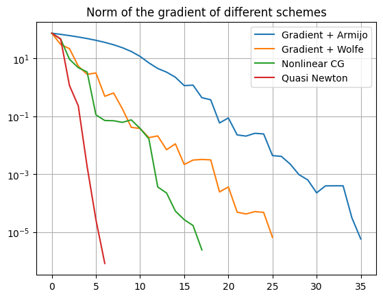
All methods converge with an absolute and relative residual norm tolerance of \(10^{-4}\). In this linear quadratic problem the Quasi Newton method with the Wolfe linesearch provides the best solution with less than 10 total number of iterations.
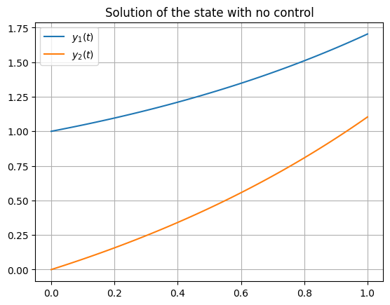
For better understanding of the problem, we plot the states \(y\) without a control function \(u\) with respect to the time \(t\).
# Plot uncontrolled state
u0 = np.zeros((data.M,data.N))
y = fun.forward(u0,data)

xAxe = np.linspace(0,data.T, num=data.N)
plt.plot(xAxe,y[0,:], label='$y_1(t)$')
plt.plot(xAxe,y[1,:], label='$y_2(t)$')
plt.title('Solution of the state with no control')
plt.grid(True)
plt.legend()
plt.show()
We will now extract the optimal solution of the results of the quasi Newton method and solve the differential equation, which is the constraint of the optimal control problem. Therefore we use the forward solver.
# Plot optimal solution
u_new_sol = np.reshape(result_quasi_newton.x, (data.M, data.N))
yfinal = fun.forward(u_new_sol,data.data)

xAxe = np.linspace(0,data.T, num=data.N)
plt.plot(xAxe,yfinal[0,:], label='$y_1(t)$')
plt.plot(xAxe,yfinal[1,:], label='$y_2(t)$')
plt.plot(xAxe,u_new_sol[0,:], label='$u_1(t)$')
plt.plot(xAxe,u_new_sol[1,:], label='$u_2(t)$')
plt.title('Optimal solution $y_1$ and $y_2$ with the optimal controls $u_1$ and $u_2$')
plt.grid(True)
plt.legend()
plt.show()
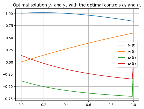
The state outcome with optimal control aligns with the desired state and desired trajectory in the cost function, since they were chosen as \(y_T=[0,1]^T\) respectively \(y_d\equiv[1,1]^T\).