Solve a box constrained optimization problem

Notebook to demonstrate how to solve an optimization problem subject to box constraints via oppy

We consider the minimization problem of the Mishra’s Bird function with box constraints

\[\begin{align*} \min_{x,y}f(x,y) = \min_{x,y}\sin(y)e^{[(1-\cos(x))^2]}+\cos(x)e^{[(1-\sin(y))^2]}+(x-y)^2, \end{align*}\]

\[\begin{align*} \mathrm{s.t.}\quad -10\leq x\leq 0 \quad \mathrm{and} \quad -6.5\leq y\leq 0. \end{align*}\]

This problem is known as a test function for optimization (see Wikipedia). The global minimum is located at

\[\begin{align*} f(-3.1302468, -1.5821422)=-106.7645367 \end{align*}\]

Firstly, we solve the problem with the projected gradient method with default linesearch i.e. with the Armijo Goldstein method. Therefore, the gradient of the Mishra’s Bird function is needed in all cases. The Mishra’s Bird and it’s gradient can be imported from the \(\small{\textbf{costfunctions.py}}\) file from the \(\small{\textbf{tests}}\) folder in the oppy package.

First we import all dependencies needed.

import numpy as np

from oppy.options import Options
from oppy.conOpt import projected_gradient

from oppy.tests.costfunctions import mishrabird, gradient_mishrabird

import matplotlib.pyplot as plt

Initial point, maximum number of iterations, lower and upper bound for the optimization methods are defined in the following:

# Initial point
x0 = np.array([-4, -2])

# Maximum number of iterations:
nmax = 1000

# lower boundaries
low = np.array([-10, -6.5])
# upper boundaries
up = np.array([0, 0])

Now we can execute the optimization algorithm and extract the residual history of each result. Furthermore we turn on the display option which shows more information in each iteration.

result_proj_grad = projected_gradient(mishrabird, gradient_mishrabird, x0, low, up,
                                         Options(disp=True))

| Iteration | Function value | Step size  |     Residual     |
| it =    1 | f =   -94.5197 | t = 0.0156 | res = 8.7467e+00 |
| it =    2 | f =   -97.3506 | t = 0.0078 | res = 3.7539e+00 |
| it =    3 | f =   -98.7256 | t = 0.0078 | res = 8.6893e+00 |
| it =    4 | f =   -99.3301 | t = 0.0078 | res = 3.7273e+00 |
| it =    5 | f =   -99.8054 | t = 0.0078 | res = 8.6728e+00 |
| it =    6 | f =  -106.7638 | t = 0.0039 | res = 6.4836e-01 |
| it =    7 | f =  -106.7645 | t = 0.0039 | res = 4.6271e-02 |
| it =    8 | f =  -106.7645 | t = 0.0039 | res = 3.3811e-03 |
| it =    9 | f =  -106.7645 | t = 0.0039 | res = 2.5231e-04 |
| Iteration | Function value | Step size  |     Residual     |
| it =   10 | f =  -106.7645 | t = 0.0039 | res = 1.9194e-05 |
| it =   11 | f =  -106.7645 | t = 0.0039 | res = 1.4841e-06 |
| it =   12 | f =  -106.7645 | t = 0.0078 | res = 1.7160e-06 |
| it =   13 | f =  -106.7645 | t = 0.0000 | res = 1.7015e-06 |
| it =   14 | f =  -106.7645 | t = 0.0039 | res = 1.3345e-07 |

The algorithm stops at a total number of iteration of 14. Another approach for faster convergence is to use another method. We try the L-BFGS-B method and thus import the algorithm. Since we use the same input as before, we can execute the algorithm right away.

from oppy.conOpt import l_bfgs_b

result_l_bfgs_b = l_bfgs_b(mishrabird, gradient_mishrabird, x0, low, up,
                                         Options(disp=True))

| Iteration | Function value | Step size  |     Residual     |
| it =    1 | f =   -35.0393 | t = 0.0156 | res = 8.7467e+00 |
| it =    2 | f =   -94.5197 | t = 0.0078 | res = 3.7539e+00 |
| it =    3 | f =   -97.3506 | t = 0.0078 | res = 6.0777e+00 |
| it =    4 | f =   -98.3201 | t = 0.0039 | res = 6.7409e-01 |
| it =    5 | f =  -106.7637 | t = 0.0039 | res = 5.7532e-01 |
| it =    6 | f =  -106.7639 | t = 1.0000 | res = 4.7448e-02 |
| it =    7 | f =  -106.7645 | t = 1.0000 | res = 6.7547e-06 |
| it =    8 | f =  -106.7645 | t = 1.0000 | res = 7.6616e-11 |

The total number of iterations is 8. For less iterations we try the projected Newton method. Therefore, we define the action of the Hessian of the Mishra’s Bird which is required for the projected Newton method and import the projected Newton and the hessian of the Mishra’s Bird function. Then we execute the projected Newton algorithm.

from oppy.conOpt import projected_newton

from oppy.tests.costfunctions import hessian_mishrabird

def action_mishrabird(u, x, Act, Inact):
    """Compute the action of the Hessian."""
    ret = Act*u + Inact*((hessian_mishrabird(x)@(Inact*u)))
    return ret

result_proj_newton = projected_newton(mishrabird, gradient_mishrabird, action_mishrabird, x0, low, up,
                                         Options(disp=True))

| Iteration | Function value | Step size  |     Residual     |
| it =    1 | f =   -94.5197 | t = 0.0156 | res = 3.2285e+00 |
| it =    2 | f =  -105.1392 | t = 1.0000 | res = 4.1891e-01 |
| it =    3 | f =  -106.7621 | t = 1.0000 | res = 1.1381e-01 |
| it =    4 | f =  -106.7645 | t = 1.0000 | res = 4.2292e-03 |
| it =    5 | f =  -106.7645 | t = 1.0000 | res = 7.0492e-07 |
| it =    6 | f =  -106.7645 | t = 1.0000 | res = 3.3995e-14 |

The projected Newton stops after 6 iterations. This result is better than the other methods. This can be compared in a residual semi y-axis log plot of the norm of the gradient with respect to the iteration number.

residual_proj_grad = result_proj_grad.res
residual_l_bfgs_b = result_l_bfgs_b.res
residual_proj_newton = result_proj_newton.res


# Plot norm of the gradient in semilogy plot
plt.semilogy(residual_proj_grad, label='proj_grad')
plt.semilogy(residual_l_bfgs_b, label='l_bfgs_b')
plt.semilogy(residual_proj_newton, label='proj_newton')
plt.title('Norm of the gradient, different schemes')
plt.grid(True)
plt.legend()
plt.show()

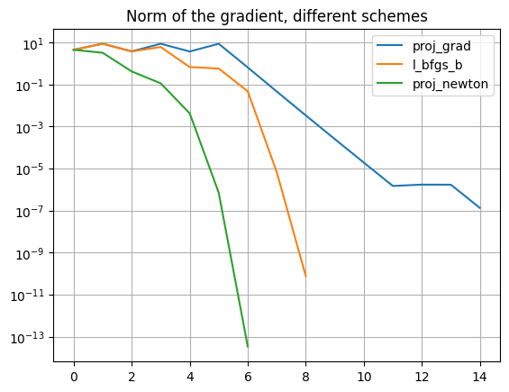
In this plot we notice that the results with the Armijo Goldstein and the projected Armijo linesearch method coincide in each optimization algorithm.

print(result_proj_grad.x)
print(result_proj_newton.x)
print(result_l_bfgs_b.x)

[-3.1302468  -1.58214218]
[-3.1302468  -1.58214218]
[-3.1302468  -1.58214218]

The results show that the solutions of the optimization methods with linesearch methods are close to the analytic global minima \((-3.1302468, -1.5821422)\), which shows a succesfull execution of the algorithms.