Solve the negative cosine problem

Introduction

In this Notebook we want to minimize the function

\[\begin{align*} -\cos : \mathbb{R} &\to \mathbb{R}\\ x &\mapsto -\cos(x) \end{align*}\]

to demonstrate the usage of the optimization package oppy. After importing all the dependencies and needed modules, we will take a quick look at the function itself and then start the minimization process.

# import several costfunctions
from oppy.tests.costfunctions import negativeCosine, gradient_negativeCosine, hessian_negativeCosine

# load standard modules
import numpy as np
import matplotlib.pyplot as plt

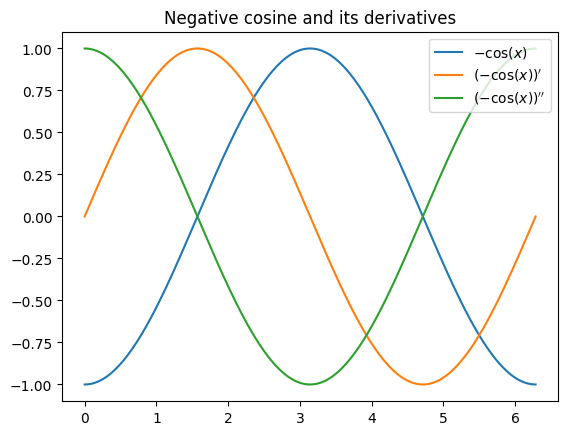
Now we will plot the function and its derivatives:

x = np.linspace(0, 2*np.pi, 200)
y = negativeCosine(x)
y_first_deriv = gradient_negativeCosine(x)
y_second_deriv = np.cos(x)

plt.plot(x,y, label="$-\cos(x)$")
plt.plot(x,y_first_deriv, label="$(-\cos(x))'$")
plt.plot(x,y_second_deriv, label="$(-\cos(x))''$")
plt.legend(loc="upper right")
plt.title("Negative cosine and its derivatives")
plt.show()

Minimization Process

Armijo and wolfe linesearch with gradient descent method

First, we need to import the linesearch algorithms, as well as the gradient descent method and the Options.

# import linesearch methods
from oppy.unconOpt import armijo, wolfe

# import optimization methods
from oppy.unconOpt import gradmethod

# import the Options class
from oppy.options import Options

In a first (and relatively simple) step, we want to minimize the negative cosine function without a lot of specified options. Afterwarts, we will manually change the options.

# set the initial/starting point
x0 = np.array([1.1655])
# inital guess, feel free to try different guesses
#x0 = np.array([1.1656])
#x0 = np.array([1.9])
#x0 = np.array([-math.atan(-math.pi)])

# show intermediate steps, while the algorithm is executed
disp = True
# use='scale' is the default, so the descent direction is always the normalized gradient
use = 'scale'

options_grad = Options(disp=disp)

Now we can test our descent method:

result_dict = {}

result_dict['res_grad'] = gradmethod(negativeCosine, gradient_negativeCosine, x0, options_grad)

# print results of the optimization process
print("x_grad = {}".format(result_dict["res_grad"].x))
print("norm gradient = {}".format(result_dict["res_grad"].res[-1]))

| Iteration | Function value | Step size  |     Residual     |
| it =    1 | f =    -0.3943 | t = 1.0000 | res = 1.6475e-01 |
| it =    2 | f =    -0.9863 | t = 0.2500 | res = 8.4399e-02 |
| it =    3 | f =    -0.9964 | t = 0.1250 | res = 4.0489e-02 |
| it =    4 | f =    -0.9992 | t = 0.0625 | res = 2.1998e-02 |
| it =    5 | f =    -0.9998 | t = 0.0312 | res = 9.2499e-03 |
| it =    6 | f =    -1.0000 | t = 0.0156 | res = 6.3750e-03 |
| it =    7 | f =    -1.0000 | t = 0.0078 | res = 1.4375e-03 |
| it =    8 | f =    -1.0000 | t = 0.0020 | res = 5.1562e-04 |
| it =    9 | f =    -1.0000 | t = 0.0010 | res = 4.6094e-04 |
| Iteration | Function value | Step size  |     Residual     |
| it =   10 | f =    -1.0000 | t = 0.0005 | res = 2.7344e-05 |
| it =   11 | f =    -1.0000 | t = 0.0000 | res = 3.1738e-06 |
| it =   12 | f =    -1.0000 | t = 0.0000 | res = 6.4087e-07 |
| it =   13 | f =    -1.0000 | t = 0.0000 | res = 3.1281e-07 |
| it =   14 | f =    -1.0000 | t = 0.0000 | res = 1.6403e-07 |
x_grad = [-1.64031982e-07]
norm gradient = 1.6403198244141418e-07

We notice that the norm of the residual is already pretty small, but we want to get faster convergence results using custom options and more advanced optimization algorithms. We start with using armijo and wolfe linesearch methods with custom options. We must prepare the inital arguments for the optimization methods: \(x_0, \gamma, \beta, \max_{\text{iter}}, c_1, c_2\) etc. We parameterize the functions with these options using the oppy.options.Options class. All of the oppy function take this class as a parameter to specify the options, but the structures and keywords can differ.

# options for the linesearch methods, feel free to try differente settings
initstep = 1
gamma = 1e-2
beta = 0.5
nmax = 30
c1 = 1e-4
c2 = 0.4

# define custom options for armijo linesearch 
options_armijo = Options(initstep=initstep, beta=beta, c1=c1, nmax=nmax)

def linesearch_armijo(x, d):
    t, flag = armijo(negativeCosine, gradient_negativeCosine, x, d, options_armijo)
    return t, flag

# define custom options for wolfe linesearch
options_wolfe = Options(initstep=initstep, c1=c1, c2=c2, beta=beta, nmax=nmax)

def linesearch_wolfe(x, d):
    t, flag = wolfe(negativeCosine, gradient_negativeCosine, x, d, options_wolfe)
    return t, flag

In a next step, we include these linesearch methods in our gradient descent method:

# armijo linesearch

options_grad_armijo = Options(disp=disp, linesearch=linesearch_armijo)

result_dict['res_grad_armijo'] = gradmethod(negativeCosine, gradient_negativeCosine, x0,
                                            options_grad_armijo)

# print results of the optimization process
print('x_grad = {}'.format(result_dict['res_grad_armijo'].x))
print('norm gradient = {}'.format(result_dict['res_grad_armijo'].res[-1]))

| Iteration | Function value | Step size  |     Residual     |
| it =    1 | f =    -0.3943 | t = 1.0000 | res = 1.6475e-01 |
| it =    2 | f =    -0.9863 | t = 0.2500 | res = 8.4399e-02 |
| it =    3 | f =    -0.9964 | t = 0.1250 | res = 4.0489e-02 |
| it =    4 | f =    -0.9992 | t = 0.0625 | res = 2.1998e-02 |
| it =    5 | f =    -0.9998 | t = 0.0312 | res = 9.2499e-03 |
| it =    6 | f =    -1.0000 | t = 0.0156 | res = 6.3750e-03 |
| it =    7 | f =    -1.0000 | t = 0.0078 | res = 1.4375e-03 |
| it =    8 | f =    -1.0000 | t = 0.0020 | res = 5.1562e-04 |
| it =    9 | f =    -1.0000 | t = 0.0010 | res = 4.6094e-04 |
| Iteration | Function value | Step size  |     Residual     |
| it =   10 | f =    -1.0000 | t = 0.0005 | res = 2.7344e-05 |
| it =   11 | f =    -1.0000 | t = 0.0000 | res = 3.1738e-06 |
| it =   12 | f =    -1.0000 | t = 0.0000 | res = 6.4087e-07 |
| it =   13 | f =    -1.0000 | t = 0.0000 | res = 3.1281e-07 |
| it =   14 | f =    -1.0000 | t = 0.0000 | res = 1.6403e-07 |
x_grad = [-1.64031982e-07]
norm gradient = 1.6403198244141418e-07

# wolfe linesearch

options_grad_wolfe = Options(disp=disp, linesearch=linesearch_wolfe)

result_dict['res_grad_wolfe'] = gradmethod(negativeCosine, gradient_negativeCosine, x0,
                                            options_grad_wolfe)

# print results of the optimization process
print('x_grad = {}'.format(result_dict['res_grad_wolfe'].x))
print('norm gradient = {}'.format(result_dict['res_grad_wolfe'].res[-1]))

| Iteration | Function value | Step size  |     Residual     |
| it =    1 | f =    -0.3943 | t = 1.0000 | res = 1.6475e-01 |
| it =    2 | f =    -0.9863 | t = 0.2500 | res = 8.4399e-02 |
| it =    3 | f =    -0.9964 | t = 0.1250 | res = 4.0489e-02 |
| it =    4 | f =    -0.9992 | t = 0.0625 | res = 2.1998e-02 |
| it =    5 | f =    -0.9998 | t = 0.0312 | res = 9.2499e-03 |
| it =    6 | f =    -1.0000 | t = 0.0156 | res = 6.3750e-03 |
| it =    7 | f =    -1.0000 | t = 0.0078 | res = 1.4375e-03 |
| it =    8 | f =    -1.0000 | t = 0.0020 | res = 5.1562e-04 |
| it =    9 | f =    -1.0000 | t = 0.0010 | res = 4.6094e-04 |
| Iteration | Function value | Step size  |     Residual     |
| it =   10 | f =    -1.0000 | t = 0.0005 | res = 2.7344e-05 |
| it =   11 | f =    -1.0000 | t = 0.0000 | res = 3.1738e-06 |
| it =   12 | f =    -1.0000 | t = 0.0000 | res = 6.4087e-07 |
| it =   13 | f =    -1.0000 | t = 0.0000 | res = 3.1281e-07 |
| it =   14 | f =    -1.0000 | t = 0.0000 | res = 1.6403e-07 |
x_grad = [-1.64031982e-07]
norm gradient = 1.6403198244141418e-07

Both linesearch methods yield similar results, so we can only improve our optimization process by using a more advanced optimzation algorith: newton’s method.

Newton’s method using armijo and wolfe linesearch

We have to load again some modules. To compare the error history and thus the convergance rate, we will keep the main options as tolerance, maximum number of iterations, etc. the same.

from oppy.unconOpt import newton
# define the options using armijo and wolfe linesearch
options_newton_armijo = Options(disp=disp, linesearch=linesearch_armijo)
options_newton_wolfe = Options(disp=disp, linesearch=linesearch_wolfe)

# armijo linesearch algorithm
result_dict["res_newton_armijo"] = newton(negativeCosine, gradient_negativeCosine, hessian_negativeCosine,
                                          x0, options_newton_armijo)
print("x_newton_armijo = {}".format(result_dict["res_newton_armijo"].x))
print("norm gradient = {}".format(result_dict["res_newton_armijo"].res[-1]))
# wolfe linesearch algorithm
result_dict["res_newton_wolfe"] = newton(negativeCosine, gradient_negativeCosine, hessian_negativeCosine,
                                         x0, options_newton_wolfe)
print("\nx_newton_wolfe = {}".format(result_dict["res_newton_wolfe"].x))
print("norm gradient = {}".format(result_dict["res_newton_wolfe"].res[-1]))

| Iteration | Function value | Step size  |     Residual     |
| it =    1 | f =    -0.3943 | t = 1.0000 | res = 9.1888e-01 |
| it =    2 | f =    -0.3945 | t = 1.0000 | res = 9.1830e-01 |
| it =    3 | f =    -0.3959 | t = 1.0000 | res = 9.1512e-01 |
| it =    4 | f =    -0.4032 | t = 1.0000 | res = 8.9744e-01 |
| it =    5 | f =    -0.4411 | t = 1.0000 | res = 7.9586e-01 |
| it =    6 | f =    -0.6055 | t = 1.0000 | res = 3.8387e-01 |
| it =    7 | f =    -0.9234 | t = 1.0000 | res = 2.1735e-02 |
| it =    8 | f =    -0.9998 | t = 1.0000 | res = 3.4239e-06 |
| it =    9 | f =    -1.0000 | t = 1.0000 | res = 1.3379e-17 |
x_newton_armijo = [-1.33793089e-17]
norm gradient = 1.3379308918355301e-17
| Iteration | Function value | Step size  |     Residual     |
| it =    1 | f =    -0.3943 | t = 1.0000 | res = 9.1888e-01 |
| it =    2 | f =    -0.3945 | t = 1.0000 | res = 9.1830e-01 |
| it =    3 | f =    -0.3959 | t = 1.0000 | res = 9.1512e-01 |
| it =    4 | f =    -0.4032 | t = 1.0000 | res = 8.9744e-01 |
| it =    5 | f =    -0.4411 | t = 1.0000 | res = 7.9586e-01 |
| it =    6 | f =    -0.6055 | t = 1.0000 | res = 3.8387e-01 |
| it =    7 | f =    -0.9234 | t = 1.0000 | res = 2.1735e-02 |
| it =    8 | f =    -0.9998 | t = 1.0000 | res = 3.4239e-06 |
| it =    9 | f =    -1.0000 | t = 1.0000 | res = 1.3379e-17 |

x_newton_wolfe = [-1.33793089e-17]
norm gradient = 1.3379308918355301e-17

We can clearly see that newton’s method converges faster and yields a more precise result.

Comparison of the different algorithms

In this step, we will extend our repertory of optmization methods by the Quasi-Newton-method and the nonlinear CG method. To do so, we need some more imports:

# import optimization methods
from oppy.unconOpt import nonlinear_cg, quasinewton

# options for nonlinear cg
options_nl_cg_wolfe = Options(disp=disp, linesearch=linesearch_wolfe)

# options for quasinewton method
options_qn_wolfe = Options(disp=disp, linesearch=linesearch_wolfe)

result_dict['res_nonlinear_cg_wolfe'] = nonlinear_cg(negativeCosine, gradient_negativeCosine, x0,
                                                     options_nl_cg_wolfe)

result_dict['res_qn_wolfe'] = quasinewton(negativeCosine, gradient_negativeCosine, x0,
                                           options_qn_wolfe)

| Iteration | Function value | Step size  |     Residual     |
| it =    1 | f =    -0.9698 | t = 1.0000 | res = 2.4403e-01 |
| it =    2 | f =    -0.9977 | t = 1.0000 | res = 6.7236e-02 |
| it =    3 | f =    -0.9999 | t = 1.0000 | res = 1.3657e-02 |
| it =    4 | f =    -1.0000 | t = 1.0000 | res = 2.2130e-03 |
| it =    5 | f =    -1.0000 | t = 1.0000 | res = 3.0050e-04 |
| it =    6 | f =    -1.0000 | t = 1.0000 | res = 3.5264e-05 |
| it =    7 | f =    -1.0000 | t = 1.0000 | res = 3.6527e-06 |
| it =    8 | f =    -1.0000 | t = 1.0000 | res = 3.3915e-07 |
| it =    9 | f =    -1.0000 | t = 1.0000 | res = 2.8567e-08 |
| Iteration | Function value | Step size  |     Residual     |
| it =    1 | f =    -0.3943 | t = 1.0000 | res = 2.4403e-01 |
| it =    2 | f =    -0.9698 | t = 1.0000 | res = 8.5631e-02 |
| it =    3 | f =    -0.9963 | t = 1.0000 | res = 5.6886e-04 |
| it =    4 | f =    -1.0000 | t = 1.0000 | res = 6.9288e-07 |
| it =    5 | f =    -1.0000 | t = 1.0000 | res = 3.7324e-14 |

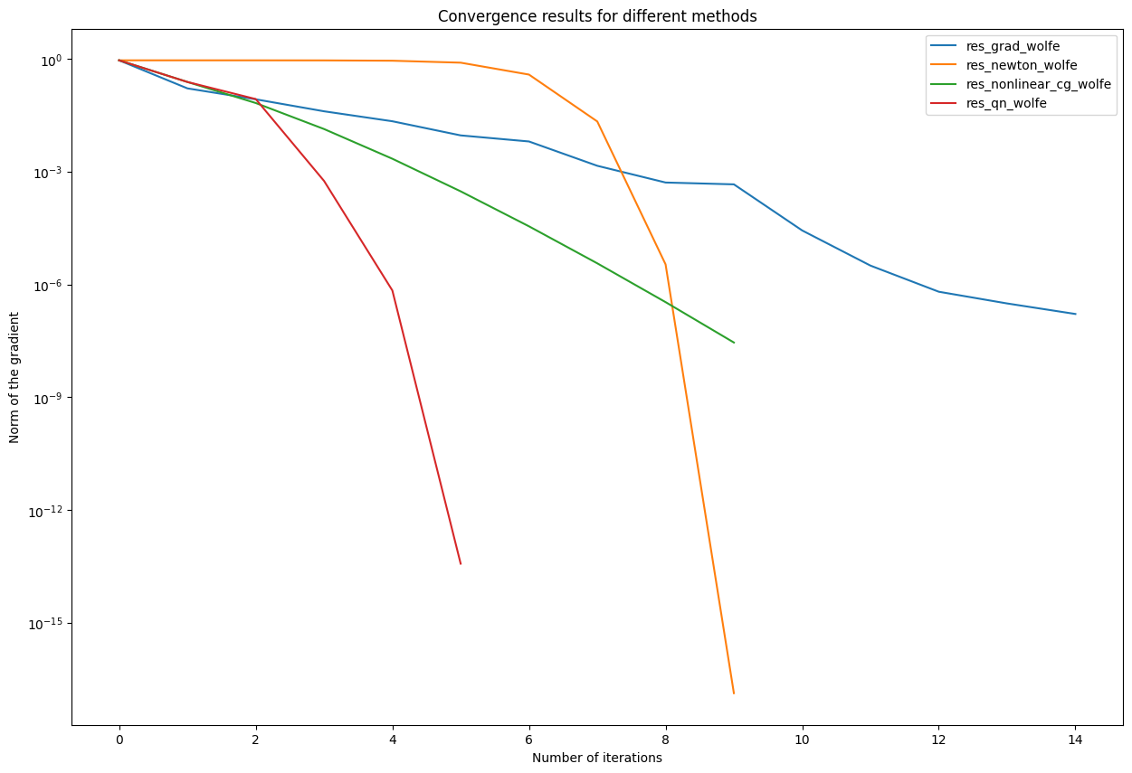
Conclusion: Comparison of convergence rates

In our last step, we compare all of the used optimization methods which used wolfe linesearch. Therefore, we need to filter our result_dict:

result_dict_wolfe = {key:value for key, value in result_dict.items() if key.endswith('wolfe')}

# plot the norm of the gradients in a semilogarithmic plot

plt.figure(figsize=(15,10))
for key in result_dict_wolfe:
    plt.semilogy(result_dict_wolfe[key].res, label = key)
plt.legend(loc="upper right")
plt.title('Convergence results for different methods')
plt.xlabel('Number of iterations')
plt.ylabel("Norm of the gradient")
plt.show()