Adjusting Parameters in a Nonlinear Model Using the Levenberg-Marquardt Method
1. Introduction
The Levenberg-Marquardt method, which is a part of the nonlinear_least_square( ) function can be used to adjust parameters of a nonlinear model such that it fits given data.
More detailed the task of adjusting parameters can be reformulated to solving a nonlinear least-squares problem:
where each \(r_j: \mathbb{R}^n \rightarrow \mathbb{R}\) stands for a residual. In our situation we further assume that every \(r_j\) is a smooth function and that \(m \geq n\) holds, which means that there are more data points than adjustable parameters.
We first look at an example, which consists of a nonlinear model as well as respective data. With this, we show how to derive the nonlinear least-squares problem and especially the objective function \(f\) which is to be minimized. Afterwards we solve the nonlinear least-squares problem by using the Levenberg-Marquardt method and obtain the adjusted model parameters.
Finally, potential problems of the Levenberg-Marquardt which might occur due to poor scaling and large residuals of the problem are discussed. Here we look at another example and modify the optional input parameters of the Levenberg-Marquardt method.
2. Example
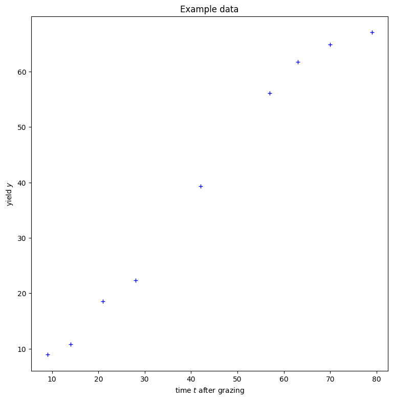
An example concerning “Pasture regrowth” presented in the book “Statistical Tools for Nonlinear Regression” by Huet et al. (2004) can be used to demonstrate the process. In the example we want to model the yield \(y\) as a nonlinear function of the time \(t\) since the last grazing. The goal is to adjust the parameters of the nonlinear function such that it fits the data.
Data:
The data points \((t_j,y_j)\) are given in the following table:
| Time after grazing \(t\) | 9 | 14 | 21 | 28 | 42 | 57 | 63 | 70 | 79 |
|---|---|---|---|---|---|---|---|---|---|
| Yield \(y\) | 8.93 | 10.8 | 18.59 | 22.33 | 39.35 | 56.11 | 61.73 | 64.92 | 67.08 |
To illustrate the problem, we can visualize the data in a scatterplot:
import matplotlib.pyplot as plt

time = [9, 14, 21, 28, 42, 57, 63, 70, 79]
yield_pasture = [8.93, 10.8, 18.59, 22.33, 39.35, 56.11, 61.73, 64.92, 67.08]

fig=plt.figure(figsize=(9, 9))
plt.xlabel("time $t$ after grazing")
plt.ylabel("yield $y$")
plt.title("Example data")
# plot the data set
plt.plot(time, yield_pasture, "b+")
plt.show()
Model:
In our example the following nonlinear model function is chosen as a model:
In summary, the goal is now to adjust the four parameters \(x_1\), \(x_2\), \(x_3\), \(x_4\). In a first step we can formulate the corresponding nonlinear least-squares problem and afterwards we use the Levenberg-Marquardt method to solve it.
Nonlinear Least-Squares Problem:
The error between a predicted model value and its respective data point is usually called the residual. In our case we get the following residuals:
In order that the model function fits best the data, the sum of the squared residuals must be minimized. Thus, we already obtain our objective function \(f\):
which is to be minimized.
3. Minimize the objective function \(f\)
The Levenberg-Marquardt method is an algorithm to solve our minimization problem. To apply it to our example, we need as inputs the residual vector and the Jacobian matrix of the residual vector. We will define them both in the first part of this section. Besides, a starting point must be chosen.
The residual vector contains all residuals of our problem \(r(x) = (r_1(x), \ldots, r_m(x))^T\). Consequently, we can calculate the residual vector directly with the model function and the given data points. The following code snippet gives us the residual vector for our example task.
import numpy as np

def model(x, t):
    return x[0]-x[1]*np.exp(-np.exp(x[2]+x[3]*np.log(t)))

def residual_vector(x):
    residuals = np.array([])
    for i in range(len(time)):
        residuals = np.append(residuals, model(x, time[i]) - yield_pasture[i])
    return residuals
A key ingredient to the Levenberg-Marquardt method is that it is using a special approximation of the Hessian of \(f(x)\), which is based on the Jacobian matrix of the residual vector \(r(x)\). This is the reason why we also have to give the Jacobian as an input to the method.
The Jacobian of the residual vector \(r(x)\) can be derived by first calculating the gradient of each residual and finally use this to build the Jacobian of the residual vector.
def gradient(x, t):
    derivation = np.array([1,-np.exp(-np.exp(x[2]+x[3]*np.log(t))),
                           -x[1]*np.exp(-np.exp(x[2]+x[3]*np.log(t)))*(-np.exp(x[2]+x[3]*np.log(t))),
                           -x[1]*np.log(t)*np.exp(-np.exp(x[2]+x[3]*np.log(t)))*(-np.exp(x[2]+x[3]*np.log(t)))])
    return derivation

def jacobian(x):
    jacobian_matrix = gradient(x, time[0])[np.newaxis, :]
    for i in np.arange(1, len(yield_pasture)):
        jacobian_matrix = np.concatenate((jacobian_matrix, gradient(x, time[i])[np.newaxis, :]), axis=0)
    return jacobian_matrix
Before we can apply the Levenberg-Marquardt method, we have to choose a starting point. In general the starting point should be chosen as close to the minimum of the objective function \(f\). Of course we do not know the minimum so the best guess can be used.
For the example we could start the iteration at:
x0 = np.array([80,70,-7,0.1])
With this we have everything together to apply the Levenberg-Marquardt method. The Levenberg-Marquardt method can be found in the nonlinear_least_square function and can be imported by the following code:
from oppy.leastSquares import nonlinear_least_square
And now it is time to start the Levenberg-Marquardt method and print the results:
result= nonlinear_least_square(residual_vector, jacobian, x0)
# print the results
print("parameter vector x = {}".format(result.x))
print("norm of the gradient of f at x = {}".format(result.res[-1]))
parameter vector x = [70.0681473  61.77265184 -9.2266518   2.38169775]
norm of the gradient of f at x = 3.99043963154179e-06
Additionaly in the default settings, “result” contains information about the iteration process, such as the number of iterations, the norm of the gradient of f at each iterate and the final iterate:
print(result)
 iterations: 12
        res: array([3.80717219e+02, 3.80717219e+02, 3.80717219e+02, 9.41868365e+03,
       4.22629857e+03, 1.12673123e+03, 6.10046372e+02, 1.96324550e+01,
       7.26078818e-01, 2.67888879e-02, 3.29284378e-04, 1.27325117e-04,
       3.99043963e-06])
          x: array([70.0681473 , 61.77265184, -9.2266518 ,  2.38169775])
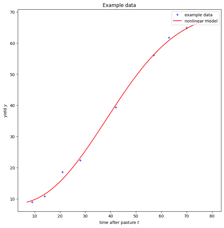
4. Graphical Illustration of the Solution
In our example it is useful to illustrate the solution by adding the nonlinear model function with its adjusted parameters into the scatterplot. This is the goal of the next code snippet.
t = np.linspace(7, 80, num=10000)
y = model(result.x,t) #solution["information"].x is our parameter vector from above

fig=plt.figure(figsize=(9, 9))
plt.xlabel("time after pasture $t$")
plt.ylabel("yield $y$")
plt.title("Example data")
plt.plot(time, yield_pasture, "b+", label="example data")
plt.plot(t,y, "r-", label="nonlinear model")
plt.legend(loc="upper right")
plt.show()
5. Potential Issues
If the Levenberg-Marquardt method has problems or fails to converge, it is usually due to poor scaling properties of the problem or that it is a large-residual problem. Poor scaling means, that a change of \(x\) in a given direction leads to a large variation in the model function, whereas a change in another direction leads to only a small variation. The Levenberg-Marquardt method contains a scaling option which should be used in this situation. When large residuals occur around the minimizer of the objective function, the underlying approximation in the algorithm is problematic which results in a slow convergence.
Poor Scaling - Example
When poor scaling occurs, the scaling option of the Levenberg-Marquardt method can be set to true. Consequently the algorithm reflects (approximately) the scaling properties of the underlying problem. Therefore we take a look at the example about the Feulgen hydrolysis kinetics, given in the book “Numerische Mathematik 1: eine algorithmisch orientierte Einführung” by Peter Deuflhard and Andreas Hohmann (2019).
Data and Model function:
The residuals are given by:
\( r_j(x) = x_1 \exp(-(x_2^2+x_3^2)t_j) \frac{\sinh((x_3^2)t_j)}{x_3^2}-y_j\),
in the example. The data \(t_j\) and \(y_j\) are given in the following code:
# Data
# at each time point t_j one value y_j is measured
time = []
for i in range(1, 31):
    time.append(6*i)

measured = [24.19, 35.34, 43.43, 42.63, 49.92, 51.53,
            57.39, 59.56, 55.60, 51.91, 58.27, 62.99,
            52.99, 53.83, 59.37, 62.35, 61.84, 61.62,
            49.64, 57.81, 54.79, 50.38, 43.85, 45.16,
            46.72, 40.68, 35.14, 45.47, 42.40, 55.21] #y

# Model function
def model(x, t):
        return x[0]*np.exp(-(x[1]**2+x[2]**2)*t)*np.sinh((x[2]**2)*t)/(x[2]**2)
In a next step we can define the residual vector and its Jacobian matrix.
# Define gradient of the residual
def gradient(x, t):
    derivative = np.array([np.exp(-(x[1] ** 2 + x[2] ** 2) * t) * np.sinh((x[2] ** 2) * t) / (x[2] ** 2),
                 -2 * x[0] * x[1] * t * np.exp(-(x[1] ** 2 + x[2] ** 2) * t) * np.sinh((x[2] ** 2) * t) / (x[2] ** 2),
                 2 * x[0] * np.exp(-(x[1] ** 2 + x[2] ** 2) * t) * (((x[2] ** 2) * t)
                                * np.cosh((x[2] ** 2) * t) - (x[2]**2 * t + 1) * np.sinh((x[2] ** 2) * t)) / (x[2] ** 3)])

    return derivative

# import functions to compute the residual vector and its Jacobian easily
from oppy.tests.costfunctions import (data_least_square,
                                      gradient_data_least_square)
# calculate the residual
def residual_vector(x):
    return data_least_square(x, model, time, measured)
# calculate the Jacobian
def jacobian(x):
    return gradient_data_least_square(x, gradient, time, measured)
The problem seems to be poorly scaled, a change in the direction \(x_2\) has a larger effect than a change in the direction \(x_1\) in the model function and thus in the respective objective function. Poor scaling makes the Levenberg-Marquardt method slow, as it results in only small steps. When we start with a starting value close to the minimizer the problem might not be problematic as the reduced step sizes might still be adequate.
# easy starting point, close to the minimizer
x0 = np.array([8, 0.055, 0.21])
result = nonlinear_least_square(residual_vector, jacobian, x0)
print(result)
 iterations: 7
        res: array([3.46101552e+05, 1.68977989e+05, 4.71404990e+04, 1.96347796e+01,
       2.44746612e+00, 4.84398756e-01, 1.07098764e-01, 2.37301401e-02])
          x: array([3.53555297, 0.05457972, 0.15385759])
However, if we start the iteration further away from the minimizer the Levenberg-Marquardt method fails to converge in our example.
# difficult starting point, further away from the minimizer
x0 = 5 * np.array([8, 0.055, 0.21])
result = nonlinear_least_square(residual_vector, jacobian, x0) # fails to converge
# after 500 steps the minimizer is not found
print("last iterate x = {}".format(result.x))
print("norm of the gradient of f at x = {}".format(result.res[-1]))
Warning: overflow encountered in sinh
Warning: invalid value encountered in double_scalars
last iterate x = [40.     0.275  1.05 ]
norm of the gradient of f at x = 11378.21529105905
Note that the two warning messages above are because the residual function is not valid on the whole domain, as the value gets too large which results in an overflow. However, this does not affect the iteration, as the Levenberg-Marquardt method is able to choose a different step in this case.
The key to solving this problem is to use the scaling option, as it is demonstrated in the next code snippet:
# import Options
from oppy.options import Options

# set the options
options = Options(scaling = True)

# apply the Levenberg-Marquardt method with the scaling option
result = nonlinear_least_square(residual_vector, jacobian, x0, options)
print(result)
 iterations: 37
        res: array([1.13782153e+04, 1.13782153e+04, 1.01645362e+05, 8.57702298e+02,
       8.57702298e+02, 8.57702298e+02, 4.54605209e+02, 7.62627925e+01,
       1.74580043e+02, 1.34164126e+03, 2.51485998e+03, 3.42453558e+02,
       3.04701232e+02, 6.21450615e+02, 2.33247724e+03, 7.87031508e+03,
       7.87031508e+03, 1.75019899e+03, 1.07993184e+04, 1.07993184e+04,
       7.02603780e+03, 1.17706227e+04, 1.17706227e+04, 4.18225479e+03,
       1.59452948e+04, 1.59452948e+04, 4.31120349e+03, 1.71811269e+04,
       1.82602693e+04, 7.20487219e+02, 4.61431148e+01, 8.06674358e+00,
       1.63258641e+00, 3.54644760e-01, 7.83232428e-02, 1.73630868e-02,
       3.85237351e-03, 8.54892052e-04])
          x: array([3.53554784, 0.05457979, 0.15385739])
To sum up, when poor scaling properties are given in the underlying problem, the Levenberg-Marquardt method cannot make large enough steps and might fail to converge within 500 steps. Nevertheless, the option “scaling” should be used, such that the scaling properties are included and the algorithm still converges.
Large Residuals - Example
In general large residuals imply that an underlying approximation which is used to find a new step in the Levenberg-Marquardt method is inappropriate. Consequently we cannot expect a fast convergence rate and the algorithm might even fail to converge. Unfortunately, there is no option available to improve the algorithm in this case. If the Levenberg-Marquardt method fails to converge, a good idea would be to choose a Newton or quasi-Newton method as they can be found in the unconstrained algorithms within the oppy package.
In the following example, the large-residual problem created by Brown and Dennis (1971) in “New computational algorithms for minimizing a sum of squares of nonlinear functions” is used. As it can be seen, the Levenberg-Marquardt method still converges to the minimizer, so the application of Newton or quasi-Newton methods is not necessary.
The residuals are given by:
where \(t_j = 0.2j\) and \(j \in \{1,\ldots,20\}\).
The following code examples apply the Levenberg-Marquardt method to this problem.
t = []
for i in range(1,21):
    t.append(i*0.2)

def residual_vector(x):  # define residuals
    residuals = np.array([])
    for i in range(len(t)):
        residuals = np.append(residuals, ((x[0]+x[1]*t[i]-np.exp(t[i]))**2+(x[2]+x[3]*np.sin(t[i])-np.cos(t[i]))**2))
    return residuals


def gradient(x, t):
    derivation = np.array([2*(x[0]+x[1]*t-np.exp(t)),
                           2*t*(x[0]+x[1]*t-np.exp(t)),
                           2*(x[2]+x[3]*np.sin(t)-np.cos(t)),
                           2*np.sin(t)*(x[2]+x[3]*np.sin(t)-np.cos(t))])
    return derivation

def jacobian(x):
    jacobian_matrix = gradient(x, t[0])[np.newaxis, :]
    for i in np.arange(1, len(t)):
        jacobian_matrix = np.concatenate((jacobian_matrix, gradient(x, t[i])[np.newaxis, :]), axis=0)
    return jacobian_matrix
Now it is time to apply the Levenberg-Marquardt method, as a start iterate we choose this time:
x0 = np.array([25,5,-5,1])
results = nonlinear_least_square(residual_vector, jacobian, x0)
print(results)
 iterations: 29
        res: array([1.04581410e+06, 1.04581410e+06, 1.04581410e+06, 1.05802632e+05,
       4.30446129e+04, 4.30446129e+04, 2.25856232e+04, 8.65289676e+03,
       8.65289676e+03, 5.82147053e+03, 1.00616726e+03, 1.00616726e+03,
       1.00616726e+03, 7.54493066e+02, 7.54493066e+02, 3.37163819e+02,
       1.35344960e+02, 1.35344960e+02, 5.72967794e+01, 1.56581471e+01,
       1.56581471e+01, 1.08846594e+01, 4.54527038e+00, 2.21160049e+00,
       2.21160049e+00, 9.58830814e-01, 5.31169684e-01, 7.34379176e-01,
       3.22556613e-01, 9.65739270e-02])
          x: array([-11.59442904,  13.20362572,  -0.40340678,   0.23681612])
Here the Levenberg-Marquardt method worked fine. However, this might not always be the case. If the algorithm would not have converged, the next option would be to use a Newton or quasi-Newton method. For more information please see the tutorials about unconstrained optimization. To demonstrate the process, we will apply a quasi-Newton method.
from oppy.unconOpt.quasinewton import quasinewton

# define objective function and its gradient
def f_objective(y):
    return 1/2*np.linalg.norm(residual_vector(y))**2
def df_objective(y):
    return np.dot(np.transpose(jacobian(y)), residual_vector(y))

# apply the quasi-Newton function
result_quasinewton = quasinewton(f_objective, df_objective, x0)
print(result_quasinewton)
 iterations: 20
        res: array([1.04581410e+06, 8.06428815e+05, 3.09959360e+05, 1.53621822e+05,
       1.53999483e+05, 1.96928238e+04, 1.67774223e+04, 1.42816942e+04,
       1.24698894e+04, 1.04279846e+04, 1.20486620e+03, 7.55974437e+02,
       1.73125654e+03, 1.90562958e+03, 1.46733538e+03, 6.94430171e+02,
       1.15949176e+02, 4.45102858e+01, 1.31549576e+01, 1.21374185e+00,
       3.08625659e-02])
          x: array([-11.59444215,  13.20363127,  -0.40344227,   0.23680475])
Here we can see that the quasi-Newton method was faster than the Levenberg-Marquardt in order to solve the large-residual problem.