Linear Least squares
Prediction of house sale prices
Consider the following situation: We would like to sell our house (area \(1000 m^2\)), but we do not yet know what the market value of the house is or what price we can ask in relation to the current market situation and our neighborhood. To solve this problem we have thought of the following.
- from the sales of some surrounding houses in our neighborhood, we have created a dataset of tuples \((x,y)\), where \(x_i\) represents the size of the living area in square meters of the house \(i\) and \(y_i\) represents the corresponding achieved sales price, for \(1 \leq i \leq n\), \(n\in \mathbb{N}\).
- we assume that the house price is linearly related to the living area, i.e., approx. \(y_i = f(x_i) = \Theta_1 + \Theta_2 \cdot x_i\) for values \((\Theta_1, \Theta_2)^T \in \mathbb{R}^2\) unknown to us so far.
We now try to determine the values \(\Theta_1, \Theta_2\) based on the data we have in order to predict our selling price. This corresponds to the simplest form of a supervised learning algorithm.
First, let’s consider our dataset (this is from https://www.kaggle.com/c/house-prices-advanced-regression-techniques/data and corresponds to actual data, for simplicity’s sake we will only load the two cells price and area here, even though the data gives much more). We now want to load the data set:
import numpy as np
dataset_name = "Houses_train.csv"
data = np.genfromtxt(dataset_name, delimiter=",")

# calculate the area in square meter insted of square foot
x_area = 1/10.764 * data[1:,4]

# Euros instead of dollars
y_price = 0.93 * data[1:,80]

# clear four datapoints with way to high spreading
for i in range(0, 4):
    for i in range(0, np.size(x_area)):
        if x_area[i] >= 10000:
            x_area = np.delete(x_area, i)
            y_price = np.delete(y_price, i)
            break
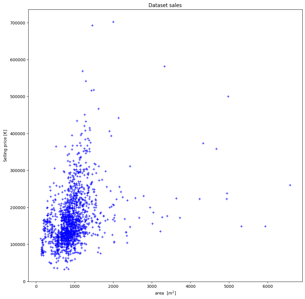
For the sake of clarity, we now present this graphically:
import matplotlib.pyplot as plt
fig=plt.figure(figsize=(12, 12))
plt.xlabel("area  $[m^2]$")
plt.ylabel("Selling price $[€]$")
plt.title("Dataset sales")
# plot the data set
plt.plot(x_area, y_price, "b+")
plt.show()
Thus, using our approach in (2), we have the following minimization problem:
Define the matrix \(A\) by
and the vector \(y\) as \(y := (y_1, \ldots , y_n)^T\) for the values from our data set. We now implement this in the code:
# calculate size of the dataset
n = np.size(x_area)
# create column vectors of ones
ones = np.ones(n)
ones_column = ones[:, np.newaxis]
# create column vectors of the dataset
x_area_column = x_area[:, np.newaxis]
# Define Matrix A
A = np.hstack((ones_column, x_area_column))
We now know that a vector \((\Theta_1, \Theta_2)^T \in \mathbb{R}^2\) solves the linear compensation problem exactly when \((\Theta_1, \Theta_2)^T\) is a solution to the normal equation
We now want to solve these by means of QR-decomposition, thus \(A = QR\) and thus it is sufficient to solve the system \(R\Theta =B\) for \(R = Q^TA\) and \(B = Q^T y\) by means of back substitution. This can be done by using oppy as follows:
from oppy.leastSquares import linear_least_square
from oppy.options import Options

# define option, using QR
opt = Options(disp=False, fargs='QR')
# solve the least squares problem
theta_sol = linear_least_square(A, y_price, opt)
print(theta_sol)
[1.21250047e+05 4.98015903e+01]
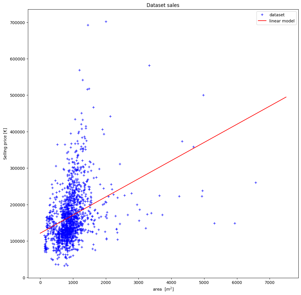
With theta_sol we now have a vector which represents the linear relationship in the data. With the function
we can now represent the straight line once graphically.
print("The straight line has the form: f(x)={1:5.2f}x + {0:5.2f}".format(theta_sol[0], theta_sol[1]))
The straight line has the form: f(x)=49.80x + 121250.05
The function \(f\) is thus a model to predict, based on our data, the purchase price of a new, previously unknown house.
x = np.linspace(0, 7500, 100000)
f_predict = lambda x: theta_sol[0] + theta_sol[1]*x
y = f_predict(x)

fig=plt.figure(figsize=(12, 12))
plt.xlabel("area  $[m^2]$")
plt.ylabel("Selling price $[€]$")
plt.title("Dataset sales")
plt.plot(x_area, y_price, "b+", label="dataset")
plt.plot(x,y, "r-", label="linear model")
plt.legend(loc="upper right")
plt.show()
Back to our initial problem: We have a house with \(1000 m^2\) area, whose purchase price we want to determine. Based on our model, we can expect the following sales price:
print("Expected selling price: {:10.2f}€".format(f_predict(1000)))
Expected selling price: 171051.64€
This gives us a simple model that gives us the expected purchase price.
Problems:
- the relationship is usually not linear.
- the target value often depends on more than one attribute (the data set has e.g. more than 80 attributes)
- the approach of a linear regression is very susceptible to individually widely scattered data points (here e.g. houses that were sold far below or above their actual price).