Solving the Rosenbrock Problem
Introduction
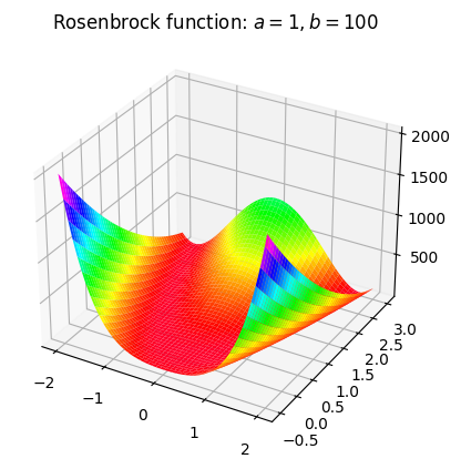
In this notebook we want to minimize the “Rosenbrock fuction”, regarding Wikipedia, the general form is given by
for \(a,b \in \mathbb{R}\). This function has a global minimum at \(x^* = (a, a^2)\) with \(f(x^*) = 0\). In our case we set \(a=1\) and \(b=100\), so the global minimum is in \((1,1)\). The function looks like this:
import numpy as np
import matplotlib.pyplot as plt
# import rosenbrock function and its derivatives
from oppy.tests.costfunctions import rosenbrock, gradient_rosenbrock, hessian_rosenbrock
# import additional plotting modules
from mpl_toolkits.mplot3d import Axes3D
from matplotlib import cm
# ==================
# surface plot
# ==================
xDef = np.linspace(-2, 2, 100)
yDef = np.linspace(-0.5, 3, 100)
X,Y = np.meshgrid(xDef, yDef)

rosenbrock_vec = lambda x,y: rosenbrock(np.array([x,y]))
Z = rosenbrock_vec(X,Y)

fig = plt.figure(1)
ax = fig.add_subplot(111, projection='3d')
surf = ax.plot_surface(X,Y,Z,cmap=cm.gist_rainbow)
plt.title("Rosenbrock function: $a=1, b=100$")
plt.show()

# ==================
# contour plot
# ==================
xDef = np.linspace(-0.5, 2, 100)
yDef = np.linspace(-0.5, 2, 100)
X,Y = np.meshgrid(xDef, yDef)

rosenbrock_vec = lambda x,y: rosenbrock(np.array([x,y]))
Z = rosenbrock_vec(X,Y)

plt.figure(2)
cp = plt.contour(X,Y,Z,np.logspace(-0.5,3.5,7,base=10),cmap=cm.coolwarm)
plt.clabel(cp, inline=True, fontsize=12)
plt.plot(1.0,1.0, "rx", label="x* = (1,1)")
plt.title("Rosenbrock function: $a=1, b=100$")
plt.legend(loc="upper right")
plt.show()
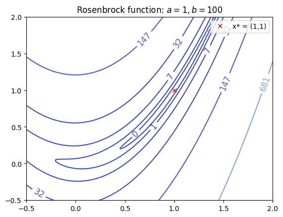
This function is pretty interesting to test our optimization algorithms, since the global minimum is inside a long, narrow, parabolic shaped flat valley. Most of the minimization methods can easily get inside this valley, but converging to the global minimum is usually pretty hard.
Minimization of the Rosenbrock function via oppy
Descent method using armijo and wolfe line search
First we need to import the missing modules:
# import line searches
from oppy.unconOpt import armijo, wolfe

# import descent method
from oppy.unconOpt import gradmethod
# import options class
from oppy.options import Options
In the first step we just want to optimize the Rosenbrock function with the descent method without a lot of specified options to get a first guess for the problem and see how it works.
#starting point:
x0 = np.array([1,-0.5])

# show intermediate steps while the algorithm is executed
disp = False
# option use=scale is default, so in the gradients method the descent direction is always normalized

# set options for line search
options_grad = Options(disp=disp)
Now we want to test our descent method:
result_dict = {}
result_dict["res_grad"] = gradmethod(rosenbrock, gradient_rosenbrock, x0, options_grad)
# print result
print("current point x = {}".format(result_dict["res_grad"].x))
print("norm gradient = {}".format(result_dict["res_grad"].res[-1]))
current point x = [0.60007213 0.36070932]
norm gradient = 0.9574691983309309
We notice that the result is not good and in this case it is what we expected, due to the complex function. In the next step we want to work with some options for the program to get a better result. We also want to use the armijo line search. Therefore we have to set some initial parameters for the minimization methods:
\(x_0, c_1, \beta, \max_{\mathrm{iter}}\). We parameterize the functions with these options using the oppy.options.Options class. All of the oppy function take this class as a parameter to specify the options, but the structures and keywords can differ.
We will try to minimize the Rosenbrock function using gradient method with armijo line search.
initstep = 1
c1 = 1e-2
# reduction parameter to reduce the stepwidth
beta = 0.5
# maximum number of iterations
nmax_line = 30
# define the options for the linesearch method
options_armijo = Options(initstep=initstep, c1=c1, nmax=nmax_line, beta=beta)

# define linesearch
def linesearch_armijo(x, d):
    t, flag = armijo(rosenbrock, gradient_rosenbrock, x, d, options_armijo)
    return t, flag
In a next step we define the options dictonary which is given to respective optimization task.
#starting point:
x0 = np.array([1,-0.5])

#maximum number of iterations for the descent method:
nmax = 100

# show intermediate steps while the algorithm is executed
disp = False
# option use=scale is default, so in the gradients method the descent direction is always normalized

# set options for line search
options_grad_armijo = Options(nmax=nmax, linesearch=linesearch_armijo, disp=disp)
Now we want to test our descent method:
result_dict["res_grad_armijo"] = gradmethod(rosenbrock, gradient_rosenbrock, x0, options_grad_armijo)
# print result
print("current point x = {}".format(result_dict["res_grad_armijo"].x))
print("norm gradient = {}".format(result_dict["res_grad_armijo"].res[-1]))
current point x = [0.61744382 0.38544152]
norm gradient = 1.9899785860076002
We can see that the result is better than in the first try but at least not good, caused by our theoretical observations from above. Maybe we have to change our line search method to wolfe line search:
c1 = 1e-4
c2 = 9/10
options_wolfe = Options(initstep=initstep, c1=c1, c2=c2, beta=beta, nmax=nmax_line)

# set options for wolfe line search
def linesearch_wolfe(x, d):
    t, flag = wolfe(rosenbrock, gradient_rosenbrock, x, d, options_wolfe)
    return t, flag

# define options for gradient method using wolfe line search
options_grad_wolfe = Options(nmax=nmax, disp=disp, linesearch=linesearch_wolfe)

result_dict["res_grad_wolfe"] = gradmethod(rosenbrock, gradient_rosenbrock, x0, options_grad_wolfe)
print("current point x = {}".format(result_dict["res_grad_wolfe"].x))
print("norm gradient = {}".format(result_dict["res_grad_wolfe"].res[-1]))
current point x = [0.60007213 0.36070932]
norm gradient = 0.9574691983309309
Although the error got slightly smaller, the result is still not really promising. Maybe we have to change some options regarding our line search. We will try it again with wolfe and we will increase the maximum amount of iterations for the line search to 200 and for the algorithm itself to 1000:
initstep = 1
# reduction parameter to reduce the stepwidth
beta = 0.5
# new maximum number of iterations for line search
nmax_line_new = 200
options_wolfe_new = Options(initstep=initstep, c1=c1, c2=c2, beta=beta, nmax=nmax_line_new)
# set options for wolfe line search
def linesearch_wolfe_new(x, d):
    t, flag = wolfe(rosenbrock, gradient_rosenbrock, x, d, options_wolfe_new)
    return t, flag
# new maximum amount of iterations for descent method
nmax_new = 1000

# define options for gradient method using wolfe line search
options_grad_wolfe_new = Options(nmax=nmax, disp=disp, linesearch=linesearch_wolfe_new)

results_grad_wolfe_new = gradmethod(rosenbrock, gradient_rosenbrock, x0, options_grad_wolfe_new)
print("current point x = {}".format(results_grad_wolfe_new.x))
print("norm gradient = {}".format(results_grad_wolfe_new.res[-1]))
current point x = [0.60007213 0.36070932]
norm gradient = 0.9574691983309309
Although the result got better, in general we do not want to have that high border for the maximum amount of iterations, because the algorithm will consume a lot of time. So we will try a more convenient optimization method: Newtons method.
Newtons method using armijo and wolfe line search
We have to load again some modules. To compare the error history and thus the convergance rate, we will keep the main options as tolerance, maximum number of iterations, etc. the same.
from oppy.unconOpt import newton
# define the options using armijo and wolfe linesearch
options_newton_armijo = Options(nmax=nmax, disp=disp, linesearch=linesearch_armijo)
options_newton_wolfe = Options(nmax=nmax, disp=disp, linesearch=linesearch_wolfe)
Let us see, how Newtons method is performing:
result_dict["res_newton_armijo"] = newton(rosenbrock, gradient_rosenbrock, hessian_rosenbrock,
                                          x0, options_newton_armijo)
print("Newton with Armijo")
print("current point x = {}".format(result_dict["res_newton_armijo"].x))
print("norm gradient = {}".format(result_dict["res_newton_armijo"].res[-1]))

result_dict["res_newton_wolfe"] = newton(rosenbrock, gradient_rosenbrock, hessian_rosenbrock,
                                         x0, options_newton_wolfe)
print("\nNewton with Wolfe")
print("current point x = {}".format(result_dict["res_newton_wolfe"].x))
print("norm gradient = {}".format(result_dict["res_newton_wolfe"].res[-1]))
Newton with Armijo
current point x = [1. 1.]
norm gradient = 0.0

Newton with Wolfe
current point x = [1. 1.]
norm gradient = 0.0
We can clearly see, that newtons method convergeces using both, armijo and wolfe, linesearch methods. The error is zero and we get our theoretical result.
Compare different optimization methods using the wolfe line search
Now we want to test some other optimization using the Rosenbrock function and compare them to each other. To keep it clear we will only use the wolfe line search and do it without the armijo line search. We will keep the same options as above.
from oppy.unconOpt import nonlinear_cg, quasinewton
# options for the fr_pr method
options_fr_wolfe = Options(nmax=nmax, disp=disp, linesearch=linesearch_wolfe)

# options for the quasinewton method
options_quasi_wolfe = Options(nmax=nmax, linesearch=linesearch_wolfe, disp=disp)

# Fletcher-Reeves-Polak-Ribiere method
result_dict["res_nonlinear_cg_wolfe"] = nonlinear_cg(rosenbrock, gradient_rosenbrock, x0, options_fr_wolfe)

# BFGS method
result_dict["res_quasi_wolfe"] = quasinewton(rosenbrock, gradient_rosenbrock, x0,
                                                   options_quasi_wolfe)
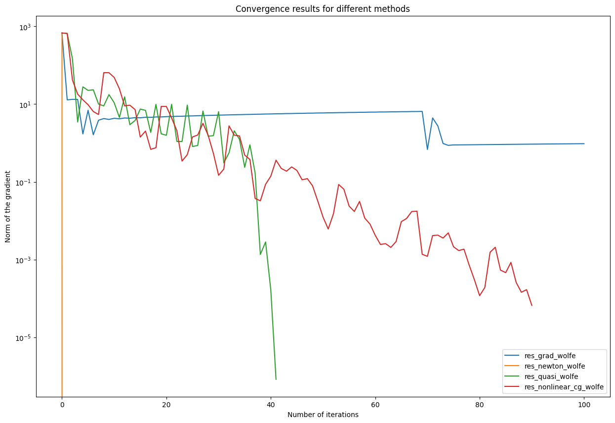
Conclusion: Comparison of convergence rates
In the cell below all results with the wolfe linesearch are printed into one graph
#==============================================================================
#Plot the norm of the gradient for all schemes:
#------------------

plt.figure(figsize=(15,10))

plt.semilogy(result_dict["res_grad_wolfe"].res, label = "res_grad_wolfe")

plt.semilogy(result_dict["res_newton_wolfe"].res, label = "res_newton_wolfe")

plt.semilogy(result_dict["res_quasi_wolfe"].res, label = "res_quasi_wolfe")

plt.semilogy(result_dict["res_nonlinear_cg_wolfe"].res, label = "res_nonlinear_cg_wolfe")

plt.legend(loc="lower right")
plt.title('Convergence results for different methods')
plt.ylabel("Norm of the gradient")
plt.xlabel('Number of iterations')
plt.show()