How to solve an integer linear program

Notebook to demonstrate the Branch and Bound Method

The example of this notebook is based on the book [1].

[1] Gerard Siersksma. Linear and Integer Programming - Theory and Practice. First Edition, Dekker 1996.

The company “CheeMi” produces besides milk mainly cheese. Part of the transport is done by the company itself, the rest has been outsourced. The current fleet of “CheeMi” is outdated and needs to be renewed. Two types of vehicles are on the shortlist. A type A vehicle can transport 100 (\(\times\) 100kg) cheese only, while a type B vehicle can transport both milk and cheese with a maximum of 50 (\(\times\) 100kg) cheese and 20 (\(\times\) 100l) milk. The purchase of a type A vehicle results in a saving of 1000 (\(\times\) 1€) per month compared to transport via an external company, while for type B it is 700 (\(\times\) 1€) per month. Of course, “CheeMi” would like to maximize its savings potential. Thus, if we denote by \(x_1\) the number of type A vehicles and by \(x_2\) the number of type B vehicles, we obtain the objective functional:

\[\begin{align*} \max 1000 x_1 + 700 x_2. \end{align*}\]

As the demand for cheese and milk is subject to regular fluctuations, the management of “CheeMi” has decided that the total capacity of vehicles to be procured should not exceed the minimum demand per day. In the case of cheese this is 2425 (\(\times\) 100kg) per day and in the case of milk this is 510 (\(\times\) 100kg) per day. This results in the following constraints:

\[\begin{align*} 100 x_1 + 50 x_2 & \leq 2425 \\ 20 x_2 & \leq 510. \end{align*}\]

Furthermore, it should be noted that the variables \(x_1\) and \(x_2\) must be integers, since it makes no sense to buy only parts of a vehicle. Thus we obtain the linear integer optimization problem “CheeMi”:

\[\begin{align*} \max & & 1000 x_1 + 700 x_2 & \\ \text{s.t.} & & 100 x_1 + 50 x_2 & \leq 2425 \\ & & 20 x_2 & \leq 510 \\ & & x_1, x_2 & \geq 0, \text{ integer}. \end{align*}\]

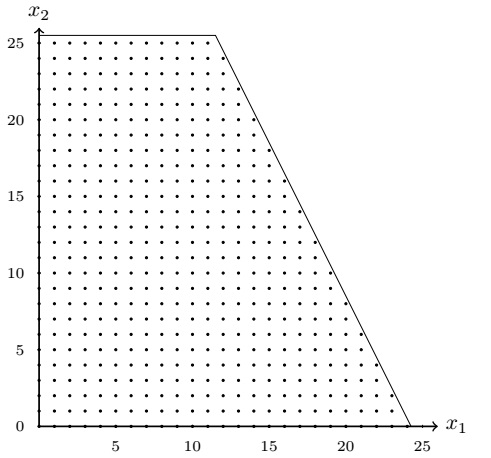
The above figure shows the admissible range. It is to be noted that the admissible range extends only over the integer points. The simplex method now finds a solution (which lies in a corner), but this solution does not have to be integer, as we can see in the picture. Simple rounding off will not suffice either. Here the optimum (if we assign the integer condition) lies in the corner \((x_1,x_2) = (11.12, 25.12)\) with maximum \(f = 29350\). If we would round up one of the components, we would leave the admissible range, rounding down yields the point \((x_1,x_2) = (11,25)\) with value of the objective function \(f = 28500\). But it is easy to see that the point \((x1,x2) = (12,24)\) reaches a higher value of the objective function (\(f= 28800\)) and is also admissible.

To solve this problem with oppy we first need to import some packages.

import numpy as np
from oppy.linOpt import b_and_b

For the method we need only the matrix A together with the vector b representing the constraints and the vector c representing the costs. With this we can solve directly.

# define matrices to solve the problem
A = np.array([[100, 50], [0, 20]])
b = np.array([2425, 510])
c = np.array([1000, 700])
# and solve it
P = b_and_b(c, A, b)
print('Optimal function value: {:.1f}'.format(P.f_opt))
print('Optimal point (x1, x2): ({:d}, {:d})'.format(int(P.x_opt[0]), int(P.x_opt[1])))
print('Number of iterations: {:d}'.format(P.iterations))

Optimal function value: 28800.0
Optimal point (x1, x2): (12, 24)
Number of iterations: 10

Here the problem with the default options was solved (see documentation for more details). Of course, we can also solve the problem with other options. One possibility would be for example

from oppy.options import Options

# set up some options
opti = Options(
        variable_search=4,       # strong branching
        initial='bestsolution',  # best solution method as init
        nodesearch='deepfirst',  # deep first algorithm inside b and b
        )
# and solve it with b and b
P = b_and_b(c, A, b)
print('Optimal function value: {:.1f}'.format(P.f_opt))
print('Optimal point (x1, x2): ({:d}, {:d})'.format(int(P.x_opt[0]), int(P.x_opt[1])))
print('Number of iterations: {:d}'.format(P.iterations))

Optimal function value: 28800.0
Optimal point (x1, x2): (12, 24)
Number of iterations: 10

Of course, this does not change the solution (although the solution vector could be different, of course), nor does it change the number of iterations needed. Nevertheless, for other problems it may be necessary to change the options.